&
!"#$%!'(()
*++%,,---#.! !$,%%!/,-'(()
)010//2*3/++/#3
4.!$506)7'
3$3/+
!"!#!$!%&#'!(!)*
+!!,,-!,./
&(0
&)1
2 &3%"30!0!& 4
0!2!

*82+ !8#+$+ #234.#29# +!/83+ # : 8+2#/;%!#2
$!// #/2 #+#3+9#89// :82+ #/+ +* 3/
!"#$%! '(()
3$3/+600)
< =05=65<00
/#$+ #82+ #/+ +*#+++/ 3/ :%!/#++/>)?(@A)??'B5+*/%%!
;%8 +/ C3/A;%!4#+ $#!+ .9 +* 82+ !8 /9/+4 # !!+ +!4# : % 8+28
#234.#29%! /#82+ !8#+$D#4%82+:!/+A !!%!2+ # :%!#2%8A$#++* !/
:% 8+2## +!.* !#+/-* E3/+.!89- ##82+ #>.!89.24+*
#234.#+B!8"89+ .;#+2 4%!.8#88 +*!-9/+ 2#+/-* .!898 /+5#/
+*!::!#+882+ !8 3+2 4/#+*#;+82+ #/* 38!%!/#++!3#234.#29#+$
*!$!// #/2 #+#3+9#89//%! //+!"#$#2+*+#234.#29*//$#:2#+FDXVDO
::2+ :!/#$+*%! ..8+9 :/3./C3#+82+ !8/322//A.9. 3+0(0+ 0(1438+ #/A
3/#$/+4+/:! 4/+!32+3!84 8 :#38 +#$.* !A4%89+*+. 3++- A+*!/ :+*
%%!#+82+ !8/322// :#234.#+/2#.++!.3++ +!/83+ # :% 8+2#/;%!#2
*C3/A;%!4#+8#89//8/ /3$$/++*+*3!/+2F:;::2+/G#F#/+!34#+8!.8G
4 8#$%%! 2*/- 38*8+ 4/8#$#:!#2/#+*/2 #+;+
%!+4#+ :2 # 42/
A!"89
1(?#/885H7''0
!"895?(=60A7''0
#
/8I2 #.!"893

1 Introduction
An essential element to the principal-agent approach to understanding politician and voter
behavior is the notion that political incumbents act in ways to raise their chances of re-election
and to further their political careers. A number of economic analyses have considered the var-
ious mechanisms through which this might occur. For example, incumbents may influence tax
and expenditure policy or monetary policy, use the office to sell political favors in exchange for
campaign contributions, or vote on legislation in a way that reflects the ideological make-up or
economic interests of their constituencies; these things are done in order to persuade voters to
support their re-election bids.
1
There is an implicit empirical prediction common to many of these
hypotheses. Winning an election, by definition, allows a politician to be the incumbent. In turn,
only an incumbent has the advantage of choosing actions available to an elected official; any non-
incumbent candidate, by definition, cannot choose these actions. Thus, if the incumbent’s actions
are meant in part to gain electoral support, then winning an election (and hence becoming the in-
cumbent) should have a reduced-form positive causal effect on the probability of being elected in
a subsequent election.
To what extent does that causal relationship hold empirically? The political science liter-
ature has been careful to recognize that answering this question, and measuring the true electoral
advantage to incumbency, is not as straightforward as the casual observer might think.
2
Through-
1
Studies that adopt a principal-agent framework in examining the political economy of elections and politician
behavior is too voluminous to review here. The following are only a few examples of studies that consider such
hypotheses. Rogoff [1990], Rogoff and Sibert [1988], and Alesina and Rosenthal [198 9] consider how incumbents
may manipulate fiscal or monetary policy to gain electoral support. Besley and Case [1995a,b] consider the tax and
expenditure-setting behavior of incumbents, and Levitt and Poterba [1994] consider how Congressional Representa-
tion might effect state econo mic growth and the geographic distribution of federal funds. Levitt [1996] considers the
relationship between constituent (and own) interests and ideology and politician voting behavior in Congress. This
is also the focus of the studies of Peltzman [1984, 1985], and Kalt and Zupan [1984]. That politicians are behaving
in a way (potentially by catering to special interests groups) to raise campaign funds, to raise re-election chances is
implicitly or explicitly examined in Levitt [1994], Grossman and Helpman [1996], Baron [1989], and Snyder [1990].
2
The empirical literature in political science that addresses the measurement of the incumbency advantage is large.
Examples of studies that consider the potential selection bias problems include Erikson[1971], Collie [1981], Garand
and Gross [1984], Jacobson [1987], Payne [1980], Alford and Hibbing [1981], and Gelman and King [1990].
1

out the latter-half of the 20th century, Representatives in the U.S. House who sought re-election
were successful about 90 percent of the time.
3
Howev e r, incumbents may enjoy re-election success
for reasons quite apart from their incumbency status. After all, there are many potential reasons
why politicians become incumbents in the first place. As one example, Democrat incumbents may
be more successful than Democratic challengers, not because there is an inherent advantage to
incumbency, but simply because Democrat incumbents tend to represent districts that are heav-
ily Democratic. In general, persistent heterogeneity across Congressional districts in the partisan
make-up of voters could, by itself, generate the observed 90 percent incumbent re-election rate.
4
No structural advantage to incumbency is needed to explain this empirical fact.
Using data on elections to the United States House of Representatives (1946-1998), this pa-
per produces quasi-experimental estimates of the true electoral advantage to political incumbency
by comparing the subsequent electoral outcomes of candidates (and their parties) that just barely
won elections to those of candidates (and their parties) that just barely lost elections. Under mild
continuity assumptions, these two groups of candidates are, as one compares closer and closer
electoral races, ex ante comparable in all other ways (on average) except in their eventual incum-
bency status. The research design approximates, to some degree, the ideal (and infeasible) classical
randomized experiment that would be needed to test the incumbency advantage hypothesis, and
hence the implicit prediction of many political agency theories. The identification strategy is rec-
ognized as an example of the regression discontinuity design, as described by Thistlethwaite and
Campbell [1960] and Campbell [1969], more recently implemented in Angrist and Lavy [1998]
and van der Klaauw [1996], and formally examined as an identification strategy in Hahn, Todd,
and van der Klaauw [2001]. In addition to providing an empirical test of the incumbency advan-
tage hypothesis, I derive a simple structural model of the individual voter’s valuation of political
3
Jacobson [1997, p. 22].
4
I sometimes refer to this alternative story as a “spurious” incumbency effect.
2

experience that permits an interpretation of the magnitude of the estimated effects.
The empirical analysis yields the following findings. First, incumbency has a significant
causal effect on the probability that a candidate (and her political party, in general) will be success-
ful in a re-election bid; it increases the probability on the order of 0.40 to 0.45.
5
The magnitude
of the effect on the two-party vote share is about 0.08. These findings are consistent with the first-
order “reduced-form” prediction of a prototypical principal-agent model of the electoral process.
6
Second, after accounting for the apparently important selection bias, losing an election reduces
the probability of running for office in the subsequent period, by about 0.43, consistent with an
enormous deterrence effect. Third, under the maintained assumptions of a particular structural
model of individual voting behavior, the estimates imply that voters place a fairly modest value
on politicians’ experience when evaluating political candidates. One additional term of Congres-
sional experience (relative to the opposing candidate) would lead to a 2 or 3 percent increase in
the vote share. On the other hand, small magnitudes in terms of the vote share can have enormous
impacts on the eventual election outcomes. A simulation using the structural estimates imply that
most (two-thirds) of the apparent electoral success rate of incumbent parties could be explained
by a political experience advantage that incumbents typically hold over their challengers. Finally,
I show evidence that in this context, an alternative “instrumental variable” approach, as well as a
“fixed effect” analysis of the same data would lead to misleading inferences.
The paper is organized as follows. Section 2 reviews the stylized facts of incumbency and
re-election in the U.S. House of Representatives in the latter half of the 20th century. Section 3
provides an illustration of how the regression discontinuity design accounts for selection bias in
testing the structural incumbency hypothesis, and establishes the continuity assumptions that are
5
As discussed below, the causal effect for the individual that I consider is the effect on the probability of both
becoming a candidate and winning the subsequent election. Below I discuss the inherent difficulty in isolating the
causal effect conditional on running for re-election.
6
For example, the framework of Austen-Smith and Banks [1989], as discussed below.
3

crucial to the research design. Section 4 reports the main reduced-form estimates of the causal
effects of incumbency. Section 5 develops a structural framework for interpreting the magnitude
of the effects in terms of the individual voter’s valuation of politicians’ experience. In section 6,
I compare the main estimates to that obtained from alternative “differencing” and “instrumental
variable” approaches to identification. Section 7 concludes.
2 The Electoral Success of Incumbents - Advantage or Artifact?
For the U.S. House of Representatives, in any given election year, the incumbent party in
a given congressional district will likely win. The solid line in Figure I shows that this re-election
rate is about 90 percent and has been fairly stable over the past 50 years.
7
Well-known in the
political science literature, the electoral success of the incumbent party is also reflectedinthe
two-party vote share, which is about 60 to 70 percent during the same period.
8
As might be expected, incumbent candidates also enjoy a high electoral success rate. Fig-
ure I shows that the winning candidate has typically had an 80 percent chance of both running for
re-election a nd ultimately winning. This is slightly lower, because the probability that an incum-
bent will be a candidate in the next election is about 88 percent, and the probability of winning,
conditional on running for election is about 90 percent. By contrast, the runner-up candidate
typically had a 3 percent chance of becoming a candidate and winning the next election. The prob-
ability that the runner-up even becomes a candidate in the next election is about 20 percent during
this period.
The casual observ er is tempted to take these figures as evidence that there is an electoral ad-
vantage to incumbency – that winning has a causal influence on the probability that the candidate
will run for office again and eventually be elected. However, the difference between the subsequent
7
Calculated from data on historical election returns from ICPSR study 7757. See Data Appendix for details. Note
that the “incumbent party” is undefined for years that end with ‘2’ due to decennial congressional re-districting.
8
See, for example, the overview in Jacobson [1997].
4
electoral outcomes of the winning and runner-up candidates may be due, perhaps entirely, to the
fact that these two groups of candidates are not ex ante comparable in important ways.
Table I illustrates the point empirically. The first row and column indicates that the winner
of any given election at time t (i.e. the incumbent for election t +1) has about a 0.803 chance of
both running in and winning election t +1. Runner-up candidates have a 0.025 percent chance.
But winning candidates prevailed over their opposition for various reasons. Perhaps they are more
charismatic, or they had more campaign resources. Another simple explanation is that voters in
the winner’s congressional district tend to vote in favor for the winner’s party, regardless of the
candidate. Wh atever the reason, it is clear from the third column of Table I that the eventual
winners of election t, are more “experienced” than the eventual runner-up candidates of election
t. In these data, even before election t is held, the eventual winners, on average, already have
served 3.798 terms in office, compared to 0.270 terms for the eventual runner-up candidates. Thus,
the difference in subsequent electoral outcomes for these two groups is perfectly c onsistent with
no effect of winning, when the candidates are ex ante non-comparable, as the empirical evidence
appears to strongly suggest.
Table I also shows that winning candidates are more likely than runner-up candidates to
become a candidate in the next election (second column). However, it is also the case that the
winning candidates were more “experienced” candidates in the first place; winning candidates of
election t have had many more attempts at gaining office than their runner-up counterparts (fourth
column). This is perfectly consiste nt with no effect of winning on the propensity to run for office
again, as long as there are systematic differences between the winners and losers of election t in
their propensities to run for election, as the data strongly suggest.
The lower part of Table I shows that whether or not candidates attempt to run again for
office, the Democratic vote-share in the next election is on average about 0.702 in districts where
5

Democrats won in election t, about 0.35 more than in the districts where the Democrat candidate
was the runner-up in election t. The interpretation of this 0.35 vote share swing as a causal effect
of the Democrats winning office is questionable, especially since the data indicate that in any given
election, winning Democratic candidates run in districts that in the past have tended to be more
favorable to Democrats, compared to their runner-up counterparts (fourth column).
9
Establishing whether or not the differences in electoral outcomes between incumbents and
non-incumbents represent a true causal effect or a simple artifact of selection is important first step
to assessing the empirical relevance of theories that adopt a principal-agent approach to model-
ing politician-voter interactions. The premise of this approach is that politicians, while in office,
strategically choose policies and actions to raise their chances of re-election, and voters discipline
the politicians’ actions with the implicit threat of voting them out of office. A finding that there is
no structural advantage to incumbency would be at odds with the predictions of theories that adopt
this framew ork.
For example, consider the model of electoral accountability and incumbency of Austen-
Smith and Banks [1989]. In this model, there are 2 identical and competing candidates, one “rep-
resentative” voter, and there are two periods. In a single period, candidates announce platforms,
the voter then chooses the candidate, the incumbent then chooses an effort level, and then there is
a random shock t hat, combined with the incumbents’ effort level, produces a policy outcome, over
which the voter’s preferences are defined. Austen-Smith and Banks show that, under certain con-
ditions, a subgame perfect Nash equilibrium arises where the threa t of dismissal (and the potential
gain to staying in office) induces the incumbent to exert effort while in office in the first period.
9
For the sake of conciseness, the rest of the empirical analysis in the paper focuses on comparing Democratic
winning candidates to Democratic losing candidates. This is done to avoid the “double-counting” of observatio ns,
since in a largely two-party context, a winning Democrat will, by construction, produce a losing Repbulican in that
district and vice versa. (It is unattractive to compare a close winner to the closer loser in the same district) In reality,
there are third-party candidates, so a parallel analysis done by focusing on Republican candidates will not give a literal
mirror image of the results. However, since third-party candidates tend not to be important in the U.S. context, it turns
out that all of the results are qualitatively the same, and are available from the author upon request.
6

The result is that the incumbent has a higher probability of winning the election in period 2, even
though the candidates are ex ante identical. A finding that there is no true electora l advantage
would be at odds with this reasonable model of electoral accountability. At the least, the finding of
no effect (or a negative effect) of incumbency should provide some reason to reconsider how we
model incumbents’ incentives and behav ior while in office.
3 Identification of the Causal Effects of Incumbency
3.1 Graphical Analysis
This paper examines the data in a way that can distinguish between the proposed causal effect
of incumbency and the artifact of pure selection. Even though winning and losing candidates are
likely to be systematically ex ante different in important ways, it i s highly plausible that winners
of elections who win by a very slim margin are likely to be ex ante comparable to candidates
who barely lose the election by a very slim margin. In the extreme case, among all political
elections that are decided by 1 vote, the winners and the losers of those elections would almost
certainly be, on average, ex ante comparable. In practice, virtually no elections are decided by
one vote. However, if the relationship between the observed vote share and subsequent electoral
outcomes is sufficiently “continuous” and “smooth”, one can estimate the average outcomes for
these hypothetical 1-vote victories and defeats, using data from cases where the margin of victory
(or defeat) is greater than 1 vote.
10
The idea of exploiting cases when a treatment variable is a
deterministic function of an observed variable in order to credibly estimate causal effects originates
in Thistlethwaite and Campbell [1960]. Here, the nature of an election (the candidate with the most
votes wins, and becomes the incumbent) provides the deterministic function, and the observed
10
Ironically, the empirical analysis may actually benefit from the fact that these extreme “photo-finish” cases are
very rare. It is easy to imagine that if all elections were decided by a handful of votes, many would be contested,
and it could be that those candidates who are better at the “post-election” battle - for recounts, for example - may be
systematically differ ent, ex ante, from those who lose the “post-election” battle.
7
variable is the vote share.
Figure IIa illustrates the regression discontinuity in the incumbency context. It plots the
estimated probability of both running in and winning election t +1as a function of the vote share
margin of victory of a candidate in elec tion t. Each point is an average of the indicator variable
for running in a nd winning election t +1for each interval, which is 0.005 wide. Points to the
left of the dashed vertical line represent subsequent electoral outcomes for the losing candidate in
election t; those to the right are for the winners.
As apparent from the figure, there is a striking discontinuous jump, right at the 0 point,
indicating that bare winners of elections are much more likely to r un for office and win the next
election than the bare losers. As long as the bare winners and bare losers are ex ante comparable
(on average) in all other ways, the difference can properly be interpreted as the causal effect of
winning election t. The causal effect is enormous: about 0.45 in probability. It is important to note
that nowhere else does a jump seem apparent. The data exhibit a well-behaved continuous and
smooth relationship between the two variables, except at the threshold that determines victory and
defeat.
Figures IIIa, IVa, and Va present the analogous pictures for three other subsequent electoral
outcomes: whether or not the candidate in election t becomes a candidate in election t +1,the
Democratic vote share (whether or not the candidate runs for re-election) in election t +1,and
whether or not the Democratic candidate (whoever it is) wins in election t +1.Allfigures exhibit
significant jumps at the threshold. They imply that the causal e ffect of winning an election is to
raise the probability of becoming a candidate in the next election by about 0.40. The incumbency
advantage for the Democratic party appears to be about 7 or 8 percent of the vote share. In terms
of the probability that the Democratic party wins the next election, the effect is about 0.35.
In all four figures, there is a noticeable positive relationship between the margin of victory
8

and the electoral outcome. For example, as shown in Figure IVa, the Democratic vote share in
election t is positively associated with the Democratic vote share in election t +1, both before and
after the threshold. This provides a sense of the importance of “selection bias”. Clearly, comparing
the means of the outcome variables between the left and right-hand side of the threshold yields
severely biased measures of the incumbency advantage. Note also that in Figures IIa, IIIa, and Va,
there appears to be important curvature in the data so that a heuristic linear least squares approach,
where the outcome is regressed on a dummy variable for victory while “controlling” for the vote
share in election t, will give somewhat misleading inferences.
11
3.2 Refutability
Knowing the function that determines the status of the endogenous regressor (here, incumbency)
does not - by itself - guarantee that the gap depicted in Figures IIa, IIIa, IVa, and Va represents
a causal effect. The crucial assumption for the causal interpretation is that all observable and
unobservable pre-determined (relative to election t) characteristics that could influence election
t +1are not systematically different between the winning and losing candidates of election t.
As an example of what might invalidate the causal inference, suppose that prior to election
t, given a ny two candidates potentially running against each other, all agents knew with certainty
the exact vote count and outcome that would occur if any pair of candidates were to run against
each other. If this were the case, we might expect that those candidates who choose to become
a candidate in an election which they know they are going to lose by 1 vote, to be systematically
different from the group of candidates who choose to become a candidate in an election which
they know they are going to win by 1 vote. Perhaps these winners happen to have, o n average,
more charisma than these losers. Then, any dif ference in the average outcomes between these two
11
The exception is Figure IVa, where the relationship looks fairly linear; however this is the case as long as one
focuses on the data lying between -0.25 and 0.25 . By using only this data, suc h a heuristic regression approach can be
thought of as a non-parmaeteric local linear estimate of the gap using a bandwidth of 0.50.
9
groups in election t+1 may be entirely due to a difference in inherent “charisma” and not at all due
to the incumbency advantage. Charisma, obviously, is only one example, and there are numerous
other dimensions in which bare winners and losers in this case may be systematically different.
Outcomes of political elections, especially the ex post close ones, are likely to have im-
portant unpredictable aspects to them; the exact vote share is never thought to be known before
the election, so it is unlikely that this particular counterexample has any real-world importance.
Nevertheless, the more general point still stands: if there is a strong reason to believe that the bare
winners of election t are systematically ex ante different from the bare losers of election t,there
would be some reason to question the internal validity of the interpretation of the discontinuity
jump as a causal effect.
Ultimately, a c redible assessment of the extent to which this might be a problem relies upon
data. If bare winners and bare losers are fundamentally non-comparable, it is likely that they will
look different based on observable pre-determined characteristics, especially those characteristics
that tend to be correlated with the electoral outcomes in election t +1. Thus, this research design
is refutable, and the extent to which the pre-determined characteristics do differ is the extent to
which we should place some doubt on the internal validity of the research design
Put another way, if the regression discontinuity design is valid (bare winners and losers
are ex ante comparable in all other ways), then any pre-determined characteristics must not be
systematically different between the bare winners and losers. Bare winners and losers should have
similar levels of congressional or electoral experience. Bare winners and losers of elections should
face opposing candidates with the same level of experience. Bare winners and losers should be in
districts that have the similar levels of political strength for their party (as proxied by their party
vote share or whether their party won in a previous election t − 1). This is analogous to the strong
prediction of an experiment that randomizes treatment and control; in the randomized experiment,
10

the baseline characteristics of the experimental subjects should not be, in any ex ante observable
way, systematically different from the control subjects.
Figures IIb, IIIb, IVb, and Vb provide evidence which seems to corroborate the validity of
the regression discontinuity design in this context. There is a strong positive relationship between
the margin of victory in election t and 1) past political experienc e, 2) electoral experience (the
number of times the candidate has run for election in the past), 3) the Democratic vote share in
t − 1, and 4) whether the Democratic party won election t − 1. However, Figure IIb shows, for
example, that bare winners and losers have, on average the same amount of accumulated congres-
sional experience by time t. There are also no visible discontinuities at the threshold for electoral
experience, the previous Democratic vote share or previous victory indicator. Close winners and
losers do appear to be quite comparable along these four dimensions; these facts lend credibility
to the identificationstrategyemployedinthisstudy.
12
3.3 Reduced-form Specification: sufficient stochastic restrictions
Before presenting the detailed results from the formal estimation procedure and drawing positive
conclusions, I formally establish the stochastic assumptions sufficient for identification of the true
incumbency effect in this context.
Consider the following reduced-form econometric specification
13
VS
jt+1
= α
t+1
+ INC
jt+1
β + µ
jt+1
(1)
where VS
jt+1
is the vote share that the Democra tic Party attains in congressional district j at elec-
tion t +1. INC
jt+1
is an indicator variable for whether the Democra tic party is the “incumbent
party” for that district and election. µ
jt+1
is a stochastic error term that represents all other ob-
12
Obviously, just as it is impossible to “prove” that the rand omization “worked” in a classical randomized experi-
ment, it is also impossible to “prove” that the close winners and losers are ex ante comparable in all other ways.
13
It is “reduced-form” in the sense that at this point I do not model the indvidiual voter’s decision. I defer this to
Section
5. Also note that for ease of exposition, I abstract from the fac t that the dependent variable is bounded between
0and1.IalsoreturntotheissueinSection
5.
11

servable and unobservable determinants of the vote share, and β is the “structural” parameter of
interest – the true party incumbency effect.
14
The important point to recognize (and is the essence of the regression discontinuity design)
is that we know the deterministic function that determines incumbency status INC
jt+1
. The party
with the most votes in election t becomes the incumbent party in election t +1. This function is
INC
jt+1
=
½
1 if VS
jt
>
1
2
0 if VS
jt
<
1
2
15
(2)
The simple comparison of the t +1vote shares between the incumbent and non-incumbent
party is then
E [VS
jt+1
|INC
jt+1
=1]− E [VS
jt
|INC
jt+1
=0]=β + BIAS
t+1
(3)
where
BI AS
t+1
= E
·
µ
jt+1
|µ
jt
>
1
2
− α
t
− INC
jt
β
¸
− E
·
µ
jt+1
|µ
jt
<
1
2
− α
t
− INC
jt
β
¸
(4)
which should be recognized as a form of the canonical characterization of selection bias when
dummy variables are endogenous.
16
Rather than try to model BI AS
t+1
in terms of observable variables, the notion in the re-
gression discontinuity approach is to compare vote shares between parties that just barely became
and barely missed being the incumbent. By doing this, we obtain
E
·
VS
jt+1
|VS
jt
=
1
2
+ e
¸
− E
·
VS
jt+1
|VS
jt
=
1
2
− e
¸
= β + BI AS
∗
t
+1
(5)
where
BI AS
∗
t
+1
= E
·
µ
jt+1
|µ
jt
=
1
2
+ e − α
t
− INC
jt
β
¸
(6)
14
β is not a structural parameter in the sense that it tells us about voter preferences. I attempt to estimate such a
structural parameter in a later section. Here, β refers to the reduced-form causal effect of incumbency on the vote-
share for the party in the next election.
15
For ease of exposition, I abstract from the existence of third parties. Generalizing to account for those thrid parties
is carried out in the empirical results.
16
See Heckman [1978] .
12

−E
·
µ
jt+1
|µ
jt
=
1
2
− e − α
t
− INC
jt
β
¸
and e represents how “close” the elections in t are.
Clearly, when µ
jt+1
and µ
jt
are jointly continuously distributed, then BI AS
∗
t+1
vanishes as
e gets smaller and smaller (we examine closer and closer elections). The goal in the estimation pro-
cedure is to use the data to estimate t he limit of E
£
VS
jt+1
|VS
jt
=
1
2
+ e
¤
− E
£
VS
jt+1
|VS
jt
=
1
2
− e
¤
as e approaches 0. That µ
jt+1
and µ
jt
is jointly continuously distributed is a very weak stochastic
restriction that is implicitly standard in virtually every econometric model that models a continuous
outcome variable.
17
What makes this approach particularly appealing is that it is unnecessary to
specify assumptions about the correlation between µ
jt+1
and INC
jt+1
or between µ
jt+1
and some
candidate instrument.
4 Estimation of the Causal Effects of Incumbency
Table II illustrates that as one compares closer and closer elections, winning and losing
candidates look more similar, and suggests that the selection bias in the naive comparison of win-
ning and losing candidates can be quite large. In the first set of columns we see that the Democrats
obtain about 70 percent of the vote share in election t +1when they win office in election t,com-
pared to about 35 percent of the vote when they lose. At the same time, on average, winning
Democrats in any given election year typically have about 3.8 terms of congressional experience
and have run in about 4 elections prior to time t, compared to 0.26 terms of experience and 0.46
elections for the losing Democrats.
18
The second set of columns demonstrate that the differences remain large when focusing
17
Or models a continuous latent index. Also, note tha tthe necessary identifying assumption is much weaker. ONe
simply needs that the conditional expectation function of µ
jt+1
with respect to µ
jt
to be continuous at the point
1
2
− α
t
− INC
jt
β.
18
The “opposition” party is defined as the party (other than the Democrats) with the highest vote share in t − 1.
Almost all of the time this is the Republican party.
13
on the three-fourths of the sample in which the margin of victory is less than 50 percent of the
vote. The probability of Democrats winning election t +1remains large at 0.88 for winners in t,
compared to the 0.10 for the losers of election t. And similarly, there remains a large difference,
for example, in the average electoral experience (the number of times a candidate has run in an
election as of year t), with a difference in favor of the winners of about 3.50 attempts.
A substantial portion of the differences go away when focusing on the 10 percent of the
elections that is decided by less than 5 percent of the vote, as shown in the third set of columns
in Table II. In this sample, the average difference in political and electoral experience between
the Democratic winners and losers is about 0.65 years, much smaller than in previous columns.
However, important differences persist: the winning Democrat candidate is significantly more
likely (by about 0.14 in probability) than a losing candidate to be in a district where the Democrats
had won the election in t − 1. Moreover, the differences in all of the pre-determined characteristics
(the variables in the 3rd t hrough 8th rows) remain and are statistically significant. It is important
to recognize, however, that this is to be expected: the sample average in a narrow neighborhood of
a margin of victory of 5 percent is in general a biased e stimate of the true conditional expectation
function when that function has a nonzero slope (which it appears to have, as illustrated in Figures
II and III).
The approach in this paper is to estimate a flexible parameterization of the function leading
up to and after the threshold, in order to estimate the mean electoral outcome at the threshold from
the left and from the right. For example, I regress the Democrat vote share t +1on a 4th-order
polynomial in the margin of victory in election t, separately, for the sample of winners in election t
(3818 observations) and for the sample of losing candidates at t (2740 observations). For indicator
variables, such as whether or not the Democratic party won in t +1, I estimate a logit with a 4th
order polynomial in the margin of victory, separately, for the winners and the losers.
14

Figures II, III, IV, and V all visually demonstrate that this procedure appears to perform
reasonably well. The regression and logit predictions do seem to line up well with the local aver-
ages plotted in the figures. In particular, Figure IIIa suggests that the data ask for different kinds
of curvature on either side of the threshold.
19
The final set of columns in Table II demonstrate that this procedure makes all of the dif-
ferences in the pre-determined characteristics between the winners and losers v anish, as exactly
predicted by the assumptions of the regression discontinuity design. In the third to eighth rows, a ll
of the differences are small and statistic ally insignificant.
20
By contrast, differences in the electoral
outcome variables – the Democrat vote share and whether the Democrats win in t +1– remain
large and statistically significant. They imply a true electoral incumbency advantage of about 8
percent in terms of the vote share, and about 0.36 in the probability of winning election t +1.
If the bare winners and losers are in all other ways ex ante comparable near the discontinu-
ity threshold, then the estimated incumbency advantage is predicted to be invariant to the inclusion
(and in the way they enter) of pre-determined characteristics as covariates. Table III shows this
to be true: the results are quite robust to various specifications. Column (1) reports the estimated
incumbency effect on the vote share, when the vote share is regressed on the victory (in election
t) indicator, the quartic in the margin of victory, and their interactions. The estimate should and
does exactly match the differences in the first row of the last set of columns in Table II. Column
(2) adds to that regression the Democratic vote share in t − 1 and whether they won in t − 1.The
19
In principle, it would be more attractive to view this as a nonparametric estimation problem, where the parameter of
interest is the conditional expectation function just to the left and right of the threshold. It would also be more attractive
to utilize an automatic bandwidth selection procedure to determine the optimal amount of smoothing. However, even
the so-called “automatic” data-b ased bandwidth selection procedure for the optimal (in the MSE sense) bandwidth at
a particular point in the support of the regressor requires as an input an initial subjective smoothing parameter. See
Fan and Gijbels [1996]. An assessment of the finite-sample performance of these procedures is beyond the scope
of this study. Instead, I assume that all of the functions belong to the class of fourth order polynomial (interacted
with winner/loser) for the regressions and logits. Statistical inference is straightforward in this framework. It simply
involves estimating the standard error of parameteric predictions at the threshold.
20
This is fa vorable for the research design in the same way it would be comforting to see that the baseline character-
istics between experimental and control subjects are on average the same in a classical randomized study.
15
Democratic share in t − 1 comes in highly significant and statistically important. The coefficient
on victory in t does not change. The coefficient also does not change when the Democrat and
opposition political and electoral experience variables are included in Columns (2)-(5).
The estimated effect also remains stable when a completely different method of controlling
for pre-determined characteristics is utilized. In Column (6), the Democratic vote share t +1is
regressed on all pre-determined characteristics (variables in rows three through eight), and the dis-
continuity jump is estimated using the residuals of this initial regression as the outcome variable.
The estimated incumbency advantage remains at about 8 percent of the vote share. Finally, in
Column (7) the vote share t − 1 is subtracted from the vote share in t +1and the discontinuity
jump in that difference is examined. Again, the coef ficient remains at about 8 percent.
Column (8) reports a final specifi cation check of the regression discontinuity design and
estimation procedure. I attempt to estimate the causal effect of the impact of winning in election t
on the vote share in t − 1.Sinceweknow that the outcome of election t cannot possibly causally
effect the electoral vote share in t−1, the estimated impact should be zero. If it significantly departs
from zero, this calls into question, some aspect of the identification strategy and/or estimation
procedure. The estimated effect is essentially 0, with a fairly small estimated standard error of
0.011. All specifications in Table III were repeated for the indicator variable for a Democrat victory
in t +1as the dependent variable, and the estimated coefficient was stable across specifications at
about 0.38 and it passed the specification check of Column (8) with a coefficient of -0.005 with a
standard error of 0.033.
By way of summarizing the results, Table IV reports the estimated causal effects of incum-
bency using the three other outcome measures that were examined in Figures IIa, IIIa, IVa, and Va.
All estimates use the full specification of Column (5) in Table III. The first two entries in the top
panel show that, at the individual candidate level, winning an election increases the probability that
16

the candidate will run for office again and be successful by about 0.45 in probability. It increases
the probability of becoming a candidate in the next election by about 0.434. It is important to
emphasize that these are not simple associational correlations. They represent the kind of causal
effects – quite plausibly free of unobservable selection bias – that can strongly suggest that their
losing may have a real deterrence effect on the decision to run for office.
21
If the politician is mak-
ing an expected utility calculation, this suggests that either the perceived payoffs or probabilities
of winning (or both) shift against the runner-up quite significantly.
It is a lso important to note that since losing has an enormous impact on even attempting
to run for office, it will be virtually impossible to convincingly estimate the candidate-level in-
cumbency advantage in terms of the advantage for the individual candidates, conditional on the
candidates running again in election t, without fully understanding the unobservable process that
determines the candidate’s decision to run for office.
22
This is because we will never observe the
vote share for candidates who choose not to pursue elected office. This is analogous to the inherent
difficulty in estimating a treatment effect in a classical randomized experiment when most of the
controls drop out of the sample.
On the other hand, the fact that candidates drop out as a consequence of the outcome of the
election is, in principle, part of the incumbency advantage. Thus, using the outcome variable that
was examined in Figure IIa (the probability that a candidate both runs in and wins election t +1)
allows estimation of the combined advantage of office, and the advantage gained through deterring
candidates from even running.
Moreover , the true incumbency adv a ntage for the party in a congressional district is well-
defined, because typically some other candidate will replace any past challengers who drop out of
21
Such a possible deterrent ef fect is discussed in Le vitt and Wolfram [1997].
22
For the approaches that attempt to tackle this difficult issue, refer to the sample selection literature beginning with
e.g. Heckman [1979] and Gronau [1977].
17

politics.
23
The third and fourth entries in the top panel of Table IV indicate that the causal effect of
the Democrat winning offic e is to raise the Democrat vote share by 0.078 in the next election, and
raise the probability that the Democratic candidate will win by 0.385.
The results make clear that the electoral success of incumbents is not an artifact of se-
lection, and hence the evidence is at least broadly consistent with the reduced-form prediction of
many political agency hypotheses that incumbents successfully utilize the opportunities embodied
in elected office to gain re-election.
24
Finally, the lower panel of Table IV shows that there is little evidence that these estimated
incumbency effects vary by sub-groups defined by the amount of political experience that the
candidate possess at election t. It would be interesting to know if the incumbency advantage
diminishes or increases as we consider more and more experienced candidates. For example, a
finding that the incumbency advantage disappeared when considering candidates that have already
been in office for a number of terms would be consistent with the notion of a signaling mechanism
[Rogoff 1990], where incumbents pursue policies to signal their type (good or bad) to voters.
However, the results are somewhat mixed. While the point estimates of the incumbency effects do
appear smaller for more experienced candidates in three of the four electoral outcome measures,
it is also true that the F-test in each case fails to reject equality of the coefficients across these
sub-groups. This suggests that any empirical analysis that purports to sort out these second order
effects will require much more data than that used in this analysis.
5 An Econometric Model of Voters’ Implicit Valuation of Political
23
And ev en in the case where no candidate runs for the party, it is not unreasonable to assign “0” to the vote share
attained by the party in that district and year.
24
Strictly speaking, political agency theories have yet to explicitly model the dynamic of how a candidate within a
party is chosen, and how candidates decide to run with the expectation of ho w the party will support them. Howe v er,
ignoring those inter-party dynamics, the “agent” could be heuristically defined as the set of possible candidates for a
party within a congressio nal district, where the party in power pursues actions that are implicitly rewarded by v oters.
18

Experience
In this section I develop a simple structural model of individual voting behavior for the
purpose of providing an economic interpretation of the magnitudes of the estimates of the incum-
bency advantage. The analysis thus far has addressed the first-order, difficult issue of disentangling
a true electoral return to holding office from an obscuring unobservable selection process. This pa-
per does not attempt to make empirical conclusions about the precise mechanism by which the
incumbency advantage arises. Much richer data is required for such an endeavor.
25
Instead, I explore what kind of institutional and behavioral assumptions can be imposed
on the data in order to make statements about the nature of voter preferences within an economic
model of utility-maximizing voters. In particular, I presume (and do not test the hypothesis) that the
incumbency advantage is simply reflective of the underlying preferences of the voters for politi-
cians’ level of congressional experience, as measured by the number of terms the politician has
served in the House of Representatives. Voters directly value the ability of a politician to engage
in the legislative process, and the goal is to estimate that valuation in terms of Congressional terms
of experience. When a candidate wins an election, she will automatically have one more term of
experience than a candidate that is otherwise identical, but who lost the election. In the model, if
voters value that extra year of experience, the winning candidate, and hence incumbent, will have
an electoral advantage in the next election.
5.1
Institutional Framework
I assume a two-party system, with candidates for the House of Representatives for each party in
25
Possessing arg uably credible estimates of this incumbency advantage is a first step towards deepening our under-
standing the causal mechanisms of the electoral advantage. Given that the findings are broadly consistent with the
implications of political agency theories, it will be a fruitful avenue for research to subject these various theories to
further empirical tests – while simultaneously addressing important selection issues that typically mak e it difficult to
distinguish between association and causation. This will require detailed data on measurable politician actions: ulti-
mately we cannot empirically distinguish between v arious hypothesized mechanisms of political agency with election
returns data alone.
19
each Congressional district. In each period, the candidates can choose to run for office, and if
they choose not to run, the party always finds a replacement. Each party announces a national
party “platform” to which the candidates of each party uniformly agree. Citizens vote for the
candidates. I do not model the detailed process of how the platform arises, but I do assume that
once in office, no single politician can influence the party platform. In any given election year
t +1the Democratic platform is represented by the scalar δ
t+1
and the Republican platform by
ρ
t+1
, normalizing δ
t+1
> ρ
t+1
.
5.2 Voters
Suppose that in any congressional district j at election t +1, we can represent individual voter
i’s political preference by the scalar ε
ijt+1
; higher ε
ijt+1
represents more liberal preferences. It
is taken as exogenous, with ε
ijt+1
∼ N (a
jt+1
, 1) , so that preferences are heterogeneous within
district and year, but the location of the distribution varies arbitrarily across districts and over time.
The preferences of an individual voter is unobservable to politicians, and prior to the election
in t +1, a
jt+1
itself is unpredictable, even if politicians possess estimates or forecasts of a
jt+1
(through polls).
Assume that citizens’ v oting is influenced by only two factors: 1) the relative “closeness”
of the announced national party platforms to their own political preferences, and 2) the relative
Congressional experience ∆EXP
jt+1
(normalized as the Democrat’s political experience minus
that of the Re publican, and measured in number of Congressional terms) between the two candi-
dates.
The individual’s propensity to vote Democrat is represented by the index
γ∆EXP
jt+1
+ ε
ijt+1
(7)
with the value of candidates’ Congressional experience denoted by γ, γ > 0. The vote v
ijt+1
of
20

individual i in district j at election t +1is described by
v
ijt+1
=
½
Democrat if γ∆EXP
jt+1
+ ε
ijt+1
>
δ
t+1
+ρ
t+1
2
Republican otherwise
(8)
So, for example, if there is no political experience difference between the two candidates, voters
will choose based on which national party platform is “closer” to their own political preference.
But if ∆EXP
jt+1
> 0 (the Democratic candidate is more experienced), then individuals may
vote for the Democrat candidate, even though their positions are closer to the Republican national
platform. The reverse is true for ∆EXP
jt+1
< 0.
This voting rule, implies that the vote share obtained by the Democrat in district j at elec-
tion t +1is
VS
jt+1
= Φ
µ
γ∆EXP
jt+1
−
δ
t+1
+ ρ
t+1
2
+ a
jt+1
. (9)
VS
jt+1
and ∆EXP
jt+1
is directly observable from the available election returns data. Taking the
inverse normal cdf transformation of the vote share yields a structural equation
Φ
−1
jt+1
= Φ
−1
(VS
jt+1
)=γ∆EXP
jt+1
−
δ
t+1
+ ρ
t+1
2
+ a
jt+1
. (10)
5.3 Candidates
I do not specifically model the candidates decision to run, and the process by which they become
candidates. Thus, the econometric framework is robust to various specifications about that partic-
ular part of the process. The important point is that the decisions of the candidates of election t to
runinelectiont +1will directly affect the value of ∆EXP
jt+1
. For example, if the i ncumbent
is a Democrat and both she and her Republican challenger from election t choose to run against
each other again, then ∆EXP
jt+1
= ∆EXP
jt
+1. If the Republican retires, and is replaced
by a more inexperienced candidate, then the political experience differential will be greater than
∆EXP
jt
+1.
21

5.4 Identification
Consider estimating the following ratio, with e very small:
E
£
Φ
−1
jt+1
|VS
jt
=
1
2
+ e
¤
− E
£
Φ
−1
jt+1
|VS
jt
=
1
2
− e
¤
E
£
∆EXP
jt+1
|VS
jt
=
1
2
+ e
¤
− E
£
∆EXP
jt+1
|VS
jt
=
1
2
− e
¤
(11)
The numerator is simply the average difference in the transformed Democratic vote share in elec-
tion t +1, between bare winners and bare losers in election t. The denominator is the average
Democratic political experience advantage in election t +1, between those winners and losers in
t.
It is possible to show that this ratio equals γ, the structural parameter of interest, as long as
E
·
−
δ
t+1
+ ρ
t+1
2
+ a
jt+1
|VS
jt
=
1
2
+ e
¸
− E
·
−
δ
t+1
+ ρ
t+1
2
+ a
jt+1
|VS
jt
=
1
2
− e
¸
(12)
approaches zero as e gets arbitrarily small. This will be true if E [a
jt+1
|VS
jt
] is continuous at
VS
jt
=
1
2
– in other words, if the outcome of election t does not affect preferences a
jt+1
,which
has been assumed to be exogenous.
26
Intuitively, γ is identified by taking the ratio of two causal effects: 1) the effect of a Demo-
cratic victory in t on (a monotonic transformation of) the Democratic vote share in t+1 (which, by
assumption, operates through the voters’ valuation of experience) and 2) the effect of a Democratic
victory in t on the Democratic experience advantage in election t +1. Each of these causal effects
can be estimated using the same procedure described in Section 4
6 Structural Estimates and Alternative Estimation Approaches
Figures VIa and VIb empirically illustrate the inputs used to estimate the structural param-
eter γ. Figure VIa plots the empirical relationship between the Democratic experience advantage
26
The importance of assuming a national party platform is apparent here. If we allowed for district-specific platforms,
we might also suspect that the y could be affected by the outcome of the previous election; in that case, we could not
distinguish between v oters’ valuation of experience and the voters’ v oting in favor of the incumbent because they put
forth platforms that are more popular.
22

in t +1and the vote share margin of victory in election t.
27
The data o nce again produce a strik-
ing jump at the 0 threshold, implying that a Democratic win in t causes an experience differential
of about 2.8 congressional terms in favor of the Democratic party in t +1. We know that if all
candidates never “dropped out”, the gap would be exactly 2. The larger gap suggests that losing
Democrats (as well as the losing opposition to winning Democrats) are dropping out and being
replaced by less experienced candidates.
The discontinuous jump apparent in Figure VIb represents a causal effect of a Democratic
win in t on the (inverse normal cdf transformation of) the Democratic vote share in t +1.
28
By the
institutional and behavioral assumptions of the model, the only reason for this causal relationship
is through the effect of Democratic victory on the t +1experience differential.
The top panel of Table V reports the results from the estimation of the structural model.
In the first entry of Column (1), I estimate the “first-stage” causal effect of a Democratic win in t
on ∆EXP
jt+1
. The estimate of the denominator in Equation 11 (and the size of the discontinuity
jump in Figure VIa) is 2.832. The estimate of the numerator in Equation 11 (and the size of the
discontinuity jump in Figure VIb) is 0.208. The ratio of these values is the estimate of γ,which
is 0.073, highly statistically significant.
29
This estimate implies that an additional Congressional
term of experience (over the opposing candidate) attracts voters towards that candidate by 0.073
of a standard deviation (in terms of underlying political preferences within a district), a seemingly
modest magnitude. However, in close elections, that 0.073 translates to a 2.5 percent vote share
difference, which of course can make a significant influence on the eventual outcome.
The deceptively small estimate of γ can play a significant role accounting for the persis-
27
Local averages are calculated for every 1 percent vote share interval.
28
Since the inv erse normal cdf is unbounded, uncontested elections in t+1 were necessarily dropped. The polynomial
fits use the same 4th order polynomials in the margin of victory (interacted with victory (t)) as in previous figures.
29
Practically, this is an instrumental variable estimate from re gression of the transformed v ote share on ∆EX P
jt+1
instrumenting with the indicator of a Demo cratic win in t, using the 4th order polynomial in the margin of the victory
(and the interactio n of these terms with the win indicator) as covariates.
23

tently high electoral success of incumbents in the U.S. House. I use my estimate of γ to ask what
would the incumbent party re-election rate be if all ∆EXP
jt+1
were set to zero. This would cor-
respond to the extreme policy of mandatory term limits of 1, where in each election, no candidate
has an experience advantage. Adjusting the actual vote shares by bγ∆EXP
jt+1
and tallying up the
counterfactual electoral outcomes yields a dramatic impact. The electoral success of the incum-
bent party falls from about 90 percent to 60 percent, and the electoral success of the non-incumbent
party rises from about 10 percent to 40 percent. Approximately two-thirds of the observed electoral
success can be explained by the existing distribution of experience differences between candidates
for the U.S. House. This makes some intuitive sense, since we know (Table II) that the average po-
litical experience difference is more than 3 and a half terms of experience. The average difference
between the simulated and actual vote shares is about 10 percent, a significant political magnitude.
Finally, the bottom panel of Table V reports the estimates of the structural parameter un-
der alternative specifications: a heuristic “ fixed effects” and an alternative “instrumental variable”
approach to modeling the unobservables. An attractive feature of a research design where there
is arguably not only exogenous but also as good as random variation in the “treatment” variable,
is that it provides a baseline for assessing whether or not other c ommonly-used econometric ap-
proaches would yield the same “experimental” estimate.
30
Since “fixed effects” and “instrumental
variable” approaches implicitly assume continuity of the distribution of unobservables, the typical
assumptions used in “differencing” and IV approaches are necessarily more restrictive than the
mild stochastic assumptions invoked in Section 5. Thus, substantial deviation of the alternative es-
timates from the baseline results of Table V would be an indication t hat the assumptions required
30
This is the spirit of the influential work of Lalonde [1986]. Obviously, the situation here is not literally a con trolled,
true “experiment”. However, in a sense, there is as much evidence that this is as good as a randomized experiment
as there is, for example, that the N SW program was correctly randomized in Lalonde [1986]. This was the poin t of
showing Table II, which is analogous to Lalonde’s Table I that provides empirical evidence that the randomization
“worked”.
24

for “fixed effects” and other “IV” approaches are invalid in this particular context.
Table V show that these estimates indeed depart substantially from the quasi-experimental
estimates. A “fixed-effect” regression yields an estimate of 0.022, which is less than a third of the
magnitude of the baseline regression discontinuity estimate of γ.
31
The fixed effects assumption –
which considers 10 and assumes that a
jt+1
= a
jt
– appears to be inappropriate in this context.
Suppose the econometrician were to utilize the assumed exclusion restriction that a Demo-
cratic victory does not directly and independently impact the electoral outcome in t +1except
through ∆EXP
jt+1
. But suppose the analyst were to conjecture that there was “no reason to
belie ve that a Democratic victory should be correlated with a
jt+1
.”
32
These assumptions would
suggest an IV estimator that does not control for a non-parametric function of the margin of vic-
tory at t.
33
This analyst would obtain misleading inferences regarding γ, as shown by the last row
of estimates in Table V. This “instrumental variable” approach yields estimates that are about 50
percent too high.
In this particular application, the best estimate is in fact the simplest cross-sectional OLS
regression, which yields an estimate of about 0.06 for γ. The specification is a regression of the
transformed vote share on ∆EXP
jt+1
and a set of year dummies.
34
On the other hand, both the
OLS and alternativ e IV estimates give misleading inferences concerning whether γ varies by sub-
groups defined by ∆EXP
jt
. They imply that the γ declines with a higher initial ∆EXP
jt
, when in
fact, as the top panel of Table V demonstrates, the interaction effects are statistically insignificant.
31
This “differencing” specification is a regression of the the transformed vote share on a set of year dummies (to
presumably “absorb” the
δ
t
−ρ
t
2
term), state-district-decade dummies (that presumably “absorbs” the “permanent het-
erogeneity” in a
jt
; i.e. the assumption is that a
jt
0
= a
jt
00
for all t
0
and t
00
within a decade), and ∆EXP
jt+1
.
32
Actually, gi ven the setup of the model, there are a lot of reasons to expect that the Democrat win variable should
be correlated with a
jt+1
. Namely, a simple autocorrelation of a
jt
would produce such a correlation.
33
Specifically, the regression is the transformed vote share on ∆EXP
jt+1
using the Democratic victory indicator in
election t as an instrument, and including year dummies as the covariates.
34
This “cross-sectional OLS” specification should not be confused with the nai ve comparison of means that were
presented in Table II. Here we are examining the relationship between electoral outcomes and the experience differ-
ential.
25
The regression discontinuity estimates indicate that the null hypothesis of homogeneity along this
dimension cannot be rejected.
7 Conclusions
This paper exploits the “near”-random assignment of incumbency generated by close U.S.
House elections in order to 1) assess whether or not the electoral success of incumbents is a mere
artifact of selection, 2) quantify the reduced-form causal relationship of incumbency on subse-
quent electoral outcomes, 3) provide an input – arguably free of selection bias – to a structural
model of v oting beha vior that produces an estimate of the voter’s valuation of political experience,
and 4) to evaluate the performance of commonly-used alternative approaches to modelling the
unobservables within this context.
I find evidence that rejects the pure spurious-selection hypothesis, and estimate that incum-
bency has a significant positive causal effect on the probability that the incumbent candidate or
party will run again for office and succeed, by about 0.40 to 0.45. Losing candidates most often do
not run again for election, and while much of this is due to selection, a significant portion of this
represents a causal relationship. A structural model implies that heterogeneity in political prefer-
ences across voters (within district) is quite large, relative to the implicit valuation of congressional
experience, but that even this modest valuation can be important. According to the model, about
two-thirds of the apparent electoral success of incumbents can be attributed to the distribution of
political experience differences across Congressional districts in the U.S. Finally, the results sug-
gest that an analyst relying on a “fixed effect” approach to estimating the valuation of experie nce
would obtain a significantly downward-biased estimated. They also suggest that an analyst em-
ploying “IV” by relying on the assumed exclusion restriction – but simply asserting orthogonality
of the instrument and the unobservable error term – would generate seriously upwardly-biased
26
estimates in this particular context.
Meaningful theories of political agency ultimately make causal empirical predictions. If
there is any hope in assessing whether any or which of these theories have empirical relevance, it
lies in evaluating whether or not there is definitive evidence that these causal relationships actually
reveal themselves in real-world data. Unobservable selection and omitted-variable bias is endemic
in empirical research, so such definitive evidence is likely to be quite rare; unilaterally relying on a
particular approach (e.g. “differencing” or “IV”) for modelling unobservable mechanisms has the
potential for producing misleading inferences. By contrast, it appears that examining the “near”-
experiment generated by close elections may be a promising approach in this line of research.
27
Data Appendix
The data used for this analysis is based on the candidate-level Congressional election returns for the
U.S., from ICPSR study 7757, “Candidate and Constituency Statistics of Elections in the United
States, 1788-1990”.
The data were initially checked for internal consistencies (e.g. candidates’ vote totals not
equalling reported total vote cast), and corrected using published and official sources (Congres-
sional Quarterly [1997] and the United States House of Representatives Office of the Clerk’s Web
Page). Election returns from 1992-1998 were taken from the United States House of Representa-
tives Office of the Clerk’s Web Page, and appended to these data. Various states (e.g. Arkansas,
Louisiana, Florida, and Oklahoma) have laws that do not require the reporting of candidate vote
totals if the candidate ran unopposed. If they are the only candidate in the district, they were as-
signed a vote share of 1. Other individual missing vote totals were replaced with valid totals from
published and official sources. Individuals with more than one observation in a district year (e.g.
separate Liberal and Democrat vote totals for the same person in New York and Connecticut) were
given the total of the votes, and were assigned to the party that gave the candidate the most votes.
The name of the candidate was parsed into last name, first name, and middle names, and suffixes
such as “Jr., Sr., II, III, etc.”
Since the exact spelling of the name differs across years, the following algorithm was used
to create a unique identifier for an individual that could match the person over time. Individua ls
were first matched on state, first 5 characters of the last name, and first initial of the first name. The
second layer of the matching process isolates those with a suffix such as Jr. or Sr., and small number
of cases were hand-modified using published and official sources. This algorithm was checked by
drawing a random sample of 100 election-year-candidate observations from the original sample,
28
tracking down every separate election the individual ran in (using published and official sources;
this expanded the random sample to 517 election-year-candidate observations), and asking how
well the automatic algorithm performed. The fraction of observations from this “truth” sample
that matched with the processed data was 0.982. The fraction of the processed data for which there
was a “true” match was 0.992. Many different algorithms were tried, but the algorithm above
performed best based on the random sample.
Throughout the sample period (1946-1998), in about 3 percent of the total possible number
of elections (based on the number of seats in the House in each year), no candidate was reported
for the election. I impute the missing values using the following algorithm. Assign the state-year
a verage electoral outcome; if still missing, assign the state-decade average electoral outcome.
Two main data sets are constructed for the analysis. For all analysis at the Congressional
level, I keep all years that do not end in ‘0’ or ‘2’. This is because, strictly speaking, Congressional
districts cannot be matched between those years, due to decennial re-districting, and so in those
years, the previous or next electoral outcome is undefined. The final data set has 6558 observations.
For the analysis at the indi vidual candidate level, one can use more years, because, despite re-
districting, it is still possible to know if a candidate ran in some election, as well as the outcome.
This larger dataset has 9674 Democrat observations.
For the sake of conciseness, the empirical analysis in the paper focuses on observations for
Democrats only. This is done to avoid the “double-counting” of observations, since in a largely
two-party context, a winning Democrat will, by construction, produce a losing Republican in that
district and vice versa. (It is unattractive to compare a close winner to the closer loser in the
same district) In reality, there are third-party candidates, so a parallel analysis done by focusing
on Republican candidates will not give a literal mirror image of the results. However, since third-
party candidates tend not to be important in the U.S. context, it turns out that a ll of the results are
29
qualitatively the same, and are available from the author upon request.
30
References
[1] Alesina, Alberto, and Howard Rosenthal. “Partisan Cycles in Congressional Elections and the
Macroeconomy.” American Political Science Review 83 (1989): 373-398.
[2] Alford, John R., and John R. Hibbing. “Increased Incumbency Advantage in the House.”
Journal of Politics 43 (1981): 1042-61.
[3] Angrist, Joshua D., and Victor Lavy. “Using Maimondies’ Rule t o Estimate the Effect of Class
Size on Scholastic Achievement.” Quarterly Journal of Economics 114 (1998):533-75.
[4] Austen-Smith, David, and Jeffrey Banks. “Electoral Accountability and Incumbency.” in Mod-
els of Strategic Choice in Politics, Peter C. Ordeshook, ed. Ann Arbor, Michigan: University
of Michigan Press, 1989.
[5] Baron, David P. “Service-induced Campaign Contributions and the Electoral Equilibrium.”
Quarterly Journal of Economics 104 (1989): 45-72.
[6] Besley Timothy, and Anne Case. “Does Electoral Accountability Affect Economic Policy
Choices? Evidence from Gubernatorial Term Limits.” Quarterly Journal of Economics 110
(1995): 769-798.
[7] Besley Timothy, and Anne Case. “Incumbent Behavior: Vote-Seeking, Tax-Setting, and Yard-
stick Competition.” American Economic Review 85 (1995): 25-45.
[8] Campbell, D. T. “Reforms as Experiments.” American Psychologist 24 (1969): 409-29.
[9] Collie, Melissa P. “Incumbency, Electoral Safety, and Turnover in the House of Representa-
tives, 1952-1976.” American Political Science Review 75 (1981): 119-31.
[10] Congressional Quarterly. Congressional Elections: 1946-1996. 1997.
[11] Erikson, Robert S. “The Advantage of Incumbency in Congressional Elections.” Polity 3
(1971): 395-405.
[12] Fan, J., and I. Gijbels. Local Polynomial Modelling and Its Applications,NewYork,New
York: Chapman and Hall, 1996.
[13] Garand, James C., and Donald A. Gross. “Change in the Vote Margins for Congressional
Candidates: A Specification of the Historical Trends.” American Political Science Review 78
(1984): 17-30.
[14] Gelman, Andrew, and Gary King. “Estimating Incumbency Advantage without Bias.” Ameri-
can Journal of Political Science 34 (1990): 1142-64.
[15] Gronau, R. “Leisure, home production and work – the theory of the allocation of time revis-
ited.” Journal of Political Economy 85 (1977): 1099-1124.
[16] Grossman Gene M., and Elhanan Helpman. “Electoral Competition and Special Interest Poli-
tics.” Review of Economic Studies 63 (1996): 265-286.
[17] Hahn, Jinyong, Petra Todd, and Wilbert van der Klaauw. “Identification and Estimation of
Treatment Effects with a Regression-Discontinuity Design.” Econometrica 69 (2001): 201-
209.
[18] Heckman, James J. “Dummy Endogenous Variables in a Simultaneous Equations System.”
Econometrica 46 (1978): 931-59.
[19] Heckman, James J. “Sample selection bias as a specification error.” Econometrica 47 (1979):
153-62.
[20] Inter-university Consortium for Political and Social Research. “Candidate and Constituency
31
Statistics of Elections in the United States, 1788-1990” Computer File 5th ICPSR ed. Ann
Arbor, MI: Inter-university Consortium for Political and Social Research, producer and dis-
tributor, 1995.
[21] Jacobson, Gary C. “The Marginals Never Vanished: Incumbency and Competition in Elections
to the U.S. House of Representatives.” American Journal of Political Science 31 (1987): 126-
41.
[22] Jacobson, Gary C. The Politics of Congressional Elections, Menlo Park, California: Longman,
1997.
[23] Kalt, Joseph P., and Mark A. Zupan. “Capture and Ideology in the Economic Theory of Poli-
tics.” American Economic Review 74 (1984): 279-300.
[24] Lalonde, Robert J. “Evaluating the Econometric Evaluations of Training Programs with Ex-
perimental Data.” American Economic Review 76 (1986): 604-620.
[25] Levitt, Steven D. “Using Repeat Challengers to Estimate the Effect of Campaign Spending on
Election Outcomes in the U.S. House.” Journal of Political Economy 102 (1994): 777-798.
[26] Levitt, Steven D., and James M. Poterba. “Congressional Distributive Politics and State Eco-
nomic Performance.” NBER Working Paper #4721 (1994).
[27] Levitt, Steven D. “How Do Senators Vote? Disentangling the Role of Voter Preferences, Party
Affiliation, and Senator Ideology.” American Economic Review 86 (1996): 425-441.
[28] Levitt, Steven D., and Catherine D. Wolfram. “Decomposing the Sources of Incumbency Ad-
vantage in the U.S. House.” Legislative Studies Quarterly 22 (1997) 45-60.
[29] Payne, James L. “The Personal Electoral Advantage of House Incumbents.” American Politics
Quarterly 8 (1980): 375-98.
[30] Peltzman, Sam. “Constituent Interest a nd Congressional Voting.” Journal of Law and Eco-
nomics 27 (1984): 181-210.
[31] Peltzman, Sam. “An Economic Interpretation of the History of Congressional Voting in the
Twentieth Century.” American Economic Review 75 (1985): 656-675.
[32] Rogoff, Kenneth. “Equilibrium Political Budget Cycles.” American Economic Review 80 (1990):
21-36.
[33] Rogoff, Kenneth, and Anne Sibert. “Elections and Macroeconomic Policy Cycles” Review of
Economic Studies 55 (1988): 1-16.
[34] Snyder, James M. “Campaign Contributions as Investments: The U.S. House of Representa-
tives, 1980-1986.” Journal of Political Economy 98 (1990): 1195-1227.
[35] Thistlethwaite, D., and D. Campbell. “Regression -Discontinuity Analysis: An alternative to
the ex post facto experiment.” Journal of Educational Psychology 51 (1960): 309-17.
[36] Van der Klaauw, Wilbert. “Estimating the Effect of Financial Aid Offers on College Enroll-
ment: A Regression-Discontinuity Approach.” Unpublished manuscript (1996).
32
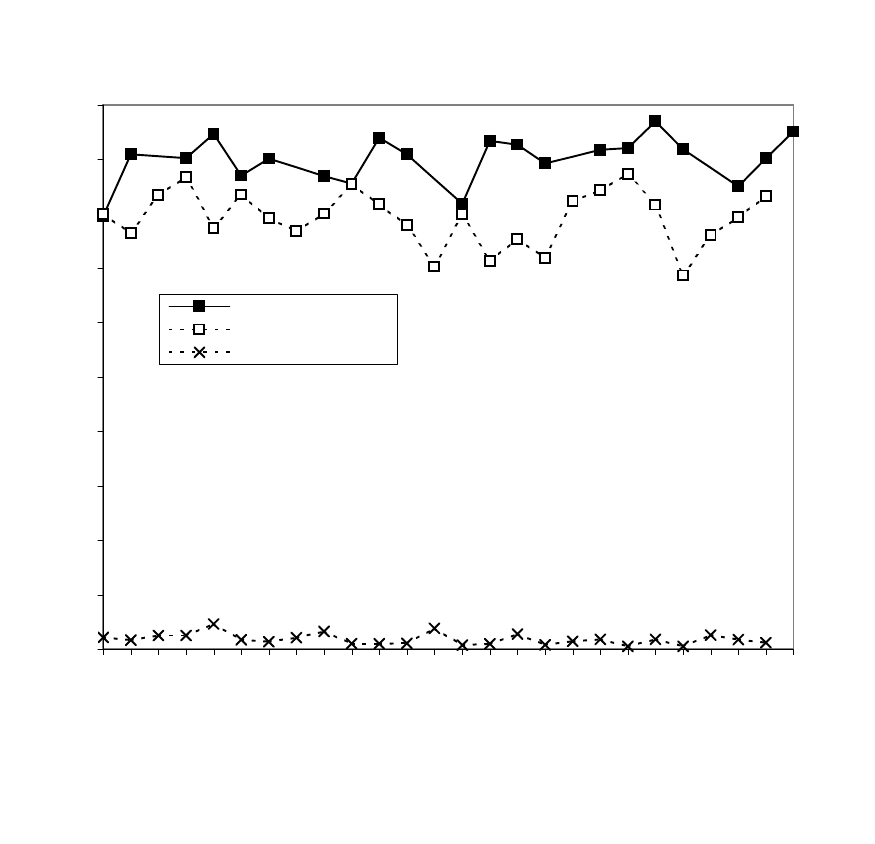
FIGURE I: Electoral Success of U.S. House Incumbents:
1948-1998
0
0.1
0.2
0.3
0.4
0.5
0.6
0.7
0.8
0.9
1
1948 1958 1968 1978 1988 1998
Year
Incumbent Party
Winning Candidate
Runner-up Candidate
Proportion Winning Election
N
ote: Calculated from ICPSR study 7757. Details in Data Appendix. Incumbent party is the party that won the election
in the preceding election in that congressional district. Due to re-districting on years that end with "2", there are no
points on those years. Other series are the fraction of individual candidates in that year, who win an election in the
following period, for both winners and runner-up candidates of that year.

0.00
0.10
0.20
0.30
0.40
0.50
0.60
0.70
0.80
0.90
1.00
-0.25 -0.20 -0.15 -0.10 -0.05 0.00 0.05 0.10 0.15 0.20 0.25
Local Average
Logit fit
Vote Share Margin of Victory, Election t
Probability of Winning, Election t+1
Figure IIa: Candidate's Probability of Winning Election t+1, by
Margin of Victory in Election t: local averages and parametric fit
0.00
0.50
1.00
1.50
2.00
2.50
3.00
3.50
4.00
4.50
5.00
-0.25 -0.20 -0.15 -0.10 -0.05 0.00 0.05 0.10 0.15 0.20 0.25
Local Average
Polynomial fit
Vote Share Margin of Victory, Election t
N
o. of Past Victories as of Election t
Figure IIb: Candidate's Accumulated Number of Past Election
Victories, by Margin of Victory in Election t: local averages and
parametric fit

0.00
0.10
0.20
0.30
0.40
0.50
0.60
0.70
0.80
0.90
1.00
-0.25 -0.20 -0.15 -0.10 -0.05 0.00 0.05 0.10 0.15 0.20 0.25
Local Average
Logit fit
Vote Share Margin of Victory, Election t
Probability of Candidacy, Election t+1
Figure IIIa: Candidate's Probability of Candidacy in Election t+1,
by Margin of Victory in Election t: local averages and parametric fit
0.00
0.50
1.00
1.50
2.00
2.50
3.00
3.50
4.00
4.50
5.00
-0.25 -0.20 -0.15 -0.10 -0.05 0.00 0.05 0.10 0.15 0.20 0.25
Local Average
Polynomial fit
Vote Share Margin of Victory, Election t
N
o. of Past Attempts as of Election t
Figure IIIb: Candidate's Accumulated Number of Past Election
Attempts, by Margin of Victory in Election t: local averages and
parametric fit

0.30
0.35
0.40
0.45
0.50
0.55
0.60
0.65
0.70
-0.25 -0.20 -0.15 -0.10 -0.05 0.00 0.05 0.10 0.15 0.20 0.25
Local Average
Polynomial fit
Vote Share Margin of Victory, Election t
Vote Share, Election t+1
Figure IVa: Democrat Party's Vote Share in Election t+1, by
Margin of Victory in Election t: local averages and parametric fit
0.30
0.35
0.40
0.45
0.50
0.55
0.60
0.65
0.70
-0.25 -0.20 -0.15 -0.10 -0.05 0.00 0.05 0.10 0.15 0.20 0.25
Local Average
Polynomial fit
Vote Share Margin of Victory, Election t
Vote Share, Election t-1
Figure IVb: Democratic Party Vote Share in Election t-1, by Margin
of Victory in Election t: local averages and parametric fit

0.00
0.10
0.20
0.30
0.40
0.50
0.60
0.70
0.80
0.90
1.00
-0.25 -0.20 -0.15 -0.10 -0.05 0.00 0.05 0.10 0.15 0.20 0.25
Local Average
Logit fit
Vote Share Margin of Victory, Election t
Probability of Victory, Election t+1
Figure Va: Democratic Party Probability Victory in Election t+1, by
Margin of Victory in Election t: local averages and parametric fit
0.00
0.10
0.20
0.30
0.40
0.50
0.60
0.70
0.80
0.90
1.00
-0.25 -0.20 -0.15 -0.10 -0.05 0.00 0.05 0.10 0.15 0.20 0.25
Local Average
Logit fit
Vote Share Margin of Victory, Election t
Probability of Victory, Election t-1
Figure Vb: Democratic Probability of Victory in Election t-1, by
Margin of Victory in Election t: local averages and parametric fit

-4.50
-3.00
-1.50
0.00
1.50
3.00
4.50
-0.25 -0.20 -0.15 -0.10 -0.05 0.00 0.05 0.10 0.15 0.20 0.25
Local Average
Polynomial fit
Vote Share Margin of Victory, Election t
Political Experience Diff. (Dem. -
Opposition), Election t+1
Figure VIa: Effect of Election Victory (t) on Political Experience
Differential (t+1)
-0.40
-0.30
-0.20
-0.10
0.00
0.10
0.20
0.30
0.40
-0.25 -0.20 -0.15 -0.10 -0.05 0.00 0.05 0.10 0.15 0.20 0.25
Local Average
Polynomial fit
Vote Share Margin of Victory, Election t
Φ
-1
(Two-party Democratic Vote Share)
Election t-1
Figure VIb: Effect of Election Victory (t) on Two-party Democratic
Vote Share Index (t+1)

TABLE I: Electoral Outcomes for Democratic Candidates and the Democratic Party,
U.S. House of Representatives, 1946-1998
Proportion Proportion a No. of Past No. of times a
Win Candidate in Victories Candidate
Election t+1 Election t+1 by Election t by Election t
Winner of Election t 0.803 0.875 3.798 3.925
(t+1 Incumbent)
Runner-up of Election t 0.025 0.186 0.270 0.479
Democratic Vote Share in Democratic Vote Share in
Election t+1 Election t-1
Winner of Election t 0.702 0.684
(t+1 Incumbent Party)
Runner-up of Election t 0.344 0.366
N
ote: Calculated from ICPSR study 7757. Details in Data Appendix. Entries are for Democratic candidates only. N=6241, 4326, 3671, and
2688 for the 1st, 2nd, 3rd, and 4th rows, respectively. The third and fourth rows exclude years that end in "2" or "0" because, due to
redistricting, voteshares in election t+1 and t-1 are not defined for those years.

Variable All |Margin|<.5 |Margin|<.05 Parametric fit
Winner Loser Winner Loser Winner Loser Winner Loser
Democrat Vote Share 0.698 0.347 0.629 0.372 0.542 0.446 0.531 0.454
Election t+1 (0.003) (0.003) (0.003) (0.003) (0.006) (0.006) (0.008) (0.008)
[0.179] [0.15] [0.145] [0.124] [0.116] [0.107]
Democrat Win Prob. 0.909 0.094 0.878 0.100 0.681 0.202 0.611 0.253
Election t+1 (0.004) (0.005) (0.006) (0.006) (0.026) (0.023) (0.039) (0.035)
[0.276] [0.285] [0.315] [0.294] [0.458] [0.396]
Democrat Vote Share 0.681 0.368 0.607 0.391 0.501 0.474 0.477 0.481
Election t-1 (0.003) (0.003) (0.003) (0.003) (0.007) (0.008) (0.009) (0.01)
[0.189] [0.153] [0.152] [0.129] [0.129] [0.133]
Democrat Win Prob. 0.889 0.109 0.842 0.118 0.501 0.365 0.419 0.416
Election t-1 (0.005) (0.006) (0.007) (0.007) (0.027) (0.028) (0.038) (0.039)
[0.31] [0.306] [0.36] [0.317] [0.493] [0.475]
Democrat Political 3.812 0.261 3.550 0.304 1.658 0.986 1.219 1.183
Experience (0.061) (0.025) (0.074) (0.029) (0.165) (0.124) (0.229) (0.145)
[3.766] [1.293] [3.746] [1.39] [2.969] [2.111]
Opposition Political 0.245 2.876 0.350 2.808 1.183 1.345 1.424 1.293
Experience (0.018) (0.054) (0.025) (0.057) (0.118) (0.115) (0.131) (0.17)
[1.084] [2.802] [1.262] [2.775] [2.122] [1.949]
Democrat Electoral 3.945 0.464 3.727 0.527 1.949 1.275 1.485 1.470
Experience (0.061) (0.028) (0.075) (0.032) (0.166) (0.131) (0.23) (0.151)
[3.787] [1.457] [3.773] [1.55] [2.986] [2.224]
Opposition Electoral 0.400 3.007 0.528 2.943 1.375 1.529 1.624 1.502
Experience (0.019) (0.054) (0.027) (0.058) (0.12) (0.119) (0.132) (0.174)
[1.189] [2.838] [1.357] [2.805] [2.157] [2.022]
Observations 3818 2740 2546 2354 322 288 3818 2740
Table II: Electoral Outcomes and Pre-determined Election Characteristics: Democratic candidates,
Winners vs. Losers: 1948-1996
N
ote: Details of data processing in Data Appendix. Estimated standard errors in parentheses. Standard deviations of variables in brackets. Data include Democratic candidates (in
election t). Democrat vote share and win probability is for the party, regardless of candidate. Political and Electoral Experience is the accumulated past election victories and election
attempts for the candidate in election t, respectively. The "opposition" party is the party with the highest vote share (other than the Democrats) in election t-1. Details of parametric fit
in text.

(1) (2) (3) (4) (5) (6) (7) (8)
Dependent Variable Vote Share Vote Share Vote Share Vote Share Vote Share Res. Vote 1st dif. Vote Vote Share
t+1 t+1 t+1 t+1 t+1 Share, t+1 Share, t+1 t-1
Victory, Election t 0.077 0.078 0.077 0.077 0.078 0.081 0.079 -0.002
(0.011) (0.011) (0.011) (0.011) (0.011) (0.014) (0.013) (0.011)
Dem. Vote Share, t-1 ---- 0.293 ---- ---- 0.298 ---- ---- ----
(0.017) (0.017)
Dem. Win, t-1 ---- -0.017 ---- ---- -0.006 ---- -0.175 0.240
(0.007) (0.007) (0.009) (0.009)
Dem. Political Experience ---- ---- -0.001 ---- 0.000 ---- -0.002 0.002
(0.001) (0.003) (0.003) (0.002)
Opp. Political Experience ---- ---- 0.001 ---- 0.000 ---- -0.008 0.011
(0.001) (0.004) (0.004) (0.003)
Dem. Electoral Experience ---- ---- ---- -0.001 -0.003 ---- -0.003 0.000
(0.001) (0.003) (0.003) (0.002)
Opp. Electoral Experience ---- ---- ---- 0.001 0.003 ---- 0.011 -0.011
(0.001) (0.004) (0.004) (0.003)
N
ote: Details of data processing in Data Appendix. N= 6558 in all regressions. Regressions include a 4th order polynomial in the margin of victory for the Democrats in Election t, with all terms interacted
with the Victory, Election t dummy variable. Political and Electoral Experience is defined in notes to Table II. Column (6) uses as its dependent variable the residuals from a least squares regression on the
Democrat Vote Share (t+1) on all the covariates. Column (7) uses as its dependent variable the Democrat Vote Share (t+1) minus the Democrat Vote Share (t-1). Column (8) uses as its dependent variable
the Democrat Vote Share (t-1). Estimated standard errors (in parentheses) are consistent with state-district-decade clustered sampling.
Table III: Effect of Winning an Election on Subsequent Party Electoral Success: Alternative Specifications, and Refutability
Test, Regression Discontinuity Estimates

Dependent Variable (t+1) Candidate Candidate Party Vote Party
Victory Candidacy Share Victory
Overall Estimate of Effect 0.450 0.434 0.078 0.385
of Victory (t) (0.031) (0.032) (0.011) (0.036)
Sub-groups, by Experience (t)
Experience=0 0.431 0.502 0.084 0.388
(0.043) (0.039) (0.013) (0.052)
Interaction: 0.027 -0.181 0.004 -0.114
0<Experience<=2 (0.104) (0.107) (0.031) (0.15)
Interaction 0.008 -0.123 -0.116 -0.249
Experience>2 (0.09) (0.115) (0.052) (0.183)
p-value 0.966 0.164 0.078 0.328
F-test of Equal Coefficients
Sample Size 9674 9674 6558 6558
Table IV: Effect of Winning an Election on Candidate Electoral Success, Candidacy,
and Party Vote Share and Electoral Success: Overall and by Experience (t) groups,
Regression Discontinuity Estimates
Note: Details of data processing in Data Appendix. Least Squares Estimates for for Democrat candidates in Election t. Estimated standard
errors (in parentheses) are consistent with candidate-levelclustering for the first two columns, and state-district-decadeclustered sampling, for
th
e
second two columns. Sub-groups defined by Political Experience as of Election t. All columns include a 4th order polynomial in the
Democratic margin of victory (with interactions with sub-groups), and Political and Electoral Experience Variables (with subgroup
interactions). Second two columns additionally include Democrat Vote Share and Victory Indicator (t-1). F-test is of the null hypothesesthat
both sub-group interactions are zero.

Regression Discontinuity Estimates
Sample Overall Exp.=0 0<Exp<=2 Exp.>2
Interaction Interaction
(1) (2) (3) (4)
First stage Relationship 2.832 2.656 -0.364 1.101
Effect of Victory on Exp. Dif. (0.311) (0.287) (0.514) (0.982)
Reduced-Form Relationship 0.208 0.222 -0.124 0.002
Effect of Victory on Vote Share (0.027) (0.032) (0.067) (0.092)
Index
Structural Parameter: Implicit 0.073 0.084 -0.041 -0.034
Value of a Year of Experience (0.012) (0.014) (0.029) (0.025)
Alternative Estimation Approaches
Cross-sectional OLS 0.060 0.052 0.032 -0.031
(0.002) (0.003) (0.012) (0.004)
"Fixed Effect" (Differencing) 0.022 0.031 0.000 -0.016
Estimator (0.003) (0.005) (0.008) (0.007)
Instrumental Variable Estimate 0.103 0.151 0.018 -0.065
(Victory in Election t as (0.002) (0.006) (0.014) (0.008)
Instrument)
Sample Size 5186 5186 ---- ----
Table V: Structural Estimation of Implicit Voters' Valuation of Political
Experience, Overall and by Experience (t) Sub-groups: Regression
Discontinuity Estimates and Alternative Estimation Approaches
Note: Details of data processingin Data Appendix. Estimates for Democrat candidates in Election t. Estimated standard errors (in
parentheses) are consistent with state-district-decade clustered sampling. Sub-groups defined by Political Experience as o
f
Election t. All regression discontinuity estimates include a 4th order polynomial in the Democratic margin of victory (t) (and
interactions with Democratic Victory (t) indicator). Details of Alternative Specifications in text.
