SAMPLING DESIGN & WEIGHTING In the original National Science

Appendix A

APPENDIX A:

SAMPLING DESIGN & WEIGHTING

In the original National Science Foundation grant, support was given for a modified probability sample. Samples for the

1972 through 1974 surveys followed this design. This modified probability design, described below, introduces the quota element at

the block level. The NSF renewal grant, awarded for the 1975-1977 surveys, provided funds for a full probability sample design, a

design which is acknowledged to be superior.

Thus, having the wherewithal to shift to a full probability sample with predesignated respondents, the 1975 and 1976 studies

were conducted with a transitional sample design, viz., one-half full probability and one-half block quota. The sample was divided

into two parts for several reasons: 1) to provide data for possibly interesting methodological comparisons; and 2) on the chance that

there are some differences over time, that it would be possible to assign these differences to either shifts in sample designs, or changes

in response patterns. For example, if the percentage of respondents who indicated that they were "very happy" increased by 10

percent between 1974 and 1976, it would be possible to determine whether it was due to changes in sample design, or an actual

increase in happiness.

There is considerable controversy and ambiguity about the merits of these two samples. Text book tests of significance

assume full rather than modified probability samples, and simple random rather than clustered random samples. In general, the

question of what to do with a mixture of samples is no easier solved than the question of what to do with the "pure" types.

Investigators who have applied statistical tests to previous General Social Survey data should continue to apply those tests.

Investigators who have refrained from applying such tests may now want to perform analyses on the probability subsample. This

would, of course, reduce the number of cases by one-half. Whatever choice investigators make, it should be remembered that the two

subsamples represent the same universe.

Having allowed for the appearance of all items in the transitional sample design, the General Social Survey then switched to

a full probability sample for the 1977, 1978, 1980, and 1982-2006 surveys. The variable SAMPLE (Col. 6973) can be used to

separate the block quota and full probability samples on the 1975 and 1976 surveys.

A similar split sample transition design was used in the 1983 survey to measure the effect of switching from the 1970 sample

frame to the 1980 sample frame. Half of the sample was drawn from the 1970 frame and half was drawn from the 1980 frame. The

variable SAMPLE (Col. 6973) separates cases from these two sample frames. Again in 1993, a split sample transition design was

employed on the 1993 survey to measure the effect of switching from the 1980 sample frame to the 1990 sample frame. Half of the

sample was drawn from each frame. In 2004 a new frame based on the 2000 census was adopted. More details on the 1970, 1980,

1990 and 2000 sample frames as well as the block quota samples appear below.

The adult, household population of the United States covered about 97.3% of the resident population of the United States in

1985. Coverage varies greatly by age group. For those 18-24, 9.4% of the population in 1980 lived outside of households (mostly in

college dorms and military quarters). Among age groups from 25 to 64 the only 0.8-1.4% of the population lived outside of

households. For those 75 and older 11.4% were in group quarters, mostly in nursing homes and long-term care facilities. For more

details on the non-household population see Living Arrangements of Children and Adults

, Census of Population, PC80-2-413, May,

1985.

Until 2006 the GSS only sampled the English speaking population. As defined for the GSS in 1983-1987, 98% of the adult,

household population is English speaking. The number of non-English speakers excluded is indicated in Table A.3. Spanish speakers

typically make up 60-65% of the language exclusions. About a dozen languages make up the remaining exclusions. Starting in 2006

the GSS sample Spanish speakers in addition to English speakers.

C. Bruce Stephenson, "Probability Sampling with Quotas: An Experiment," GSS Methodological Report No.7, April, 1979.

Published in Public Opinion Quarterly

, 43 (Winter, 1979), 477-496.

2096

Appendix A

BLOCK QUOTA

The sample is a multi-stage area probability sample to the block or segment level. At the block level, however, quota

sampling is used with quotas based on sex, age, and employment status. The cost of the quota samples is substantially less than the

cost of a full probability sample of the same size, but there is, of course, the chance of sample biases mainly due to not-at-homes

which are not controlled by the quotas. However, in order to reduce this bias, the interviewers are given instructions to canvass and

interview only after 3:00 p.m. on weekdays or during the weekend or holidays. This type of sample design is most appropriate when

the past experience and judgment of a project director suggest that sample biases are likely to be small relative to the precision of the

measuring instrument and the decisions that are to be made.

Selection of PSUs

The Primary Sampling Units (PSUs) employed are Standard Metropolitan Statistical Areas (SMSAs) or non-metropolitan

counties selected in NORC's Master Sample. These SMSAs and counties were stratified by region, age, and race before selection.

Selection of Sample within PSUs

The units of selection of the second stage were block groups (BGs) and enumeration districts (EDs). These EDs and BGs

were stratified according to race and income before selection.

The third stage of selection was that of blocks. The blocks were

selected with probabilities proportional to size. In places without block statistics, measures of size for the blocks were obtained by

field counting. The average cluster size is five respondents per cluster. This provides a suitable balance of precision and economy.

Interviewer Instructions

At the block or segment level, the interviewer begins a travel pattern at the first DU (dwelling unit) from the northwest corner

of the block and proceeds in a specified direction until the quotas have been filled.

The quotas call for approximately equal numbers of men and women with the exact proportion in each segment determined

by the 1970 Census tract data. For women, the additional requirement is imposed that there be the proper proportion of employed and

unemployed women in the location. Again, these quotas are based on the 1970 Census tract data. For men, the added requirement is

that there be the proper proportion of men over and under 35 in the location.

These particular quotas have been established because past experience has shown that employed women and young men

under 35 are the most difficult to find at home for interviewing.

Sampling Error

Although the mean squared error cannot be estimated directly from a quota sample, one can make estimates of sampling

variability using procedures such as those outlined by Stephan and McCarthy.

Past experience would suggest that, for most purposes,

this sample of 1,500 could be considered as having about the same efficiency as a simple random sample of 1,000 cases. In making

this judgment concerning the design effect, we are concerned with the "average" effect upon a large set of different variables of the

clustering of households at the last stage of selection.

Any statement of sampling error assumes that the bias in quota sampling due to

the lack of control over respondent availability is slight for the study under consideration.

For those persons interested in investigating the within-sample variability of these data, we have included a "sampling error

code" (see Q. 1523). Information about the use of this code is available from the GSS project staff at NORC.

For selection procedures, see Benjamin King and Carol Richards, "The 1972 NORC National Probability Sample." Chicago:

NORC, August, 1972.

Ibid.

Frederick Stephan and Philip McCarthy, Sampling Opinions. (New York: John Wiley and Sons, 1958, Chapter 10.)

For variable specific design effects from the 1993 GSS, see Tom W. Smith, Hee-Choon Shin, and Xiaoxi Tong, "A Report on the

Sample Frame Comparisons and Design Effects of the 1993 General Social Survey," GSS Methodological Report No. 87, 1994.

2097

Appendix A

Probability, 1970 Frame

The NORC national probability sample is a stratified, multistage area probability sample of clusters of households in the

continental United States.

The selection of geographic areas at successive stages is in accordance with the method of probabilities

proportional to size (p.p.s.). Furthermore, the clusters of households are divided into replicated subsamples in order to facilitate

estimation of the variance of sample estimators of population characteristics.

At the first stage of selection, Standard Metropolitan Statistical Areas (SMSAs) and nonmetropolitan counties covering the

total continental United States were grouped according to size strata within the nine Census regions. All population figures and other

demographic information were obtained from 1970 Census reports. Within each size stratum grouping based upon geographic

location, or racial characteristics (or both), was accomplished before selection. The final frame was further separated into zones or

"paper strata" of equal population size in order to facilitate the selection of replicated subsamples of primary sampling units (PSUs).

The selection of PSUs was designed to produce four independent subsamples of equal size. The four subsamples were randomly

combined to form two larger subsamples of 101 PSUs each.

The large subsamples are thus internally separable into two replicated

subsamples for variance estimation purposes.

NORC has selected one of the two large subsamples described above to serve as its principal frame of households for the

remainder of the decade. The PSUs fall into 89 distinct SMSAs and nonmetropolitan counties. (New York, a very large SMSA,

represents five PSUs, whereas the smaller counties represent only one PSU.)

The second-stage procedure involved the direct selection of Census block groups or enumeration districts (E.D.s) within

SMSAs or counties, eliminating the traditional intermediate stage of clustering selections within urban places or county division. The

increase in geographic dispersion within the primary areas has a negligible effect on field costs. Before selection, the Census tracts,

minor civil divisions, and Census county divisions containing the block groups and E.D.s were carefully stratified by geographic

location, income, and race, in order to maximize the precision of sample estimation within a PSU. Block groups and E.D.s were then

selected with probabilities proportional to size in numbers sufficient to satisfy survey demands for households expected throughout the

decade. Lists of the separate households contained in the second stage blocks or E.D.s were constructed by field personnel or obtained

from directories. Thus, the principal NORC national probability sample is, in effect, an inventory of identifiable households, each

with a known probability of selection. In a typical sample survey with equal probability of selection for individual households (i.e., a

self-weighting sample), households at which interviews will take place are probabilistically selected from the available lists of

addresses for blocks and E.D.s. The method of probabilities proportional to size results in the assignment of approximately equal

numbers of interviews in each final stage cluster, which in turn leads to increased precision in the estimation of overall population

characteristics.

The NORC national probability frame, with its broad geographic dispersion, its reserves of additional SMSAs and counties,

and its built-in replication, provides sufficient flexibility for application to a wide range of survey tasks. Its design is based on the

consideration of sampling problems that NORC and other organizations have encountered in past surveys, and we believe that it

substantially eliminates many of these difficulties.

Probability, 1980 Frame

1980 National Sampling Frame

The 1980 frame was designed, selected, and listed jointly by NORC and the Survey Research Center. The new frame was

selected, in most cases, in two stages; about one-fifth of the second stage units were subsampled, producing a third stage.

Eighty-four PSUs were selected at the first stage. The PSUs consist of counties, SMSAs, independent cities and, in New

England, parts of counties. Prior to selection, the United States was divided into PSUs; the PSUs were then grouped into 84 strata.

The strata were formed by grouping metropolitan and non-metropolitan PSUs within each of the four Census regions. Within each

region, additional variables were used to define strata. The stratifying variables included within-region geography and size; size was

measured by the 1980 Census count of occupied housing units. One PSU was selected from each stratum using a controlled selection

Alaska and Hawaii are not included in this sample.

The selection methods used are similar to those described in standard textbooks, e.g., W. E. Deming, Sample Design in Business

Research (New York: Wiley & Sons, 1960), and L. Kish, Survey Sampling

(New York: Wiley & Sons, 1965).

In the actual implementation of the selection method, subsamples 1 and 4 resulted in 51 PSUs, whereas subsamples 2 and 3

produced only 50 PSUs. The result was not unexpected and is due to a technical reason, details of which will be provided on request.

The inequality of subsample sizes does not affect the equal probability characteristics of the sample.

2098

Appendix A

procedure. This procedure ensured proportionate representation along certain control dimensions (such as percentage Hispanic in the

West). The exact control variables (like the stratification variables) differed somewhat from region to region. Sixteen strata contained

only one PSU, which was selected with certainty. The remaining 68 PSUs were selected with probability proportional to size

(measured in housing units).

The unit for second stage selection was the block or enumeration district (ED). The number of secondary selections within a

PSU depended in part on the stratum size. The number of second stage selections listed for NORC's national frame in the 16 PSUs

selected with certainty ranged from 24 to six selections for PSU. In the remaining 68 sample PSUs, six second stage selections were

listed. (The same number of second stage selections were listed for SRC's national frame; further, both organizations retained a

similar number of second stage selections as a reserve for future use.) All total, the new frame includes 562 secondary selections.

Prior to selection, the second stage units within each sample PSU were sorted by county, by minor civil division (in some

areas), by Census Tract or ED number, and by block number. Counties were ordered within PSUs according to size and geography

(e.g., in SMSAs, the county containing the central city came first, then counties containing nearby suburbs, and so on). In twenty

states, information was available on the size and median family income of minor civil divisions (MCDs), which are governmental

units below the county level (such as cities or towns). Where this information was available, we sorted the block and EDs by MCD

and ordered the MCDs by size and income.

Next, we sorted all blocks and EDs by Census Tract number and then by block or ED number; these sorts establish a

geographic ordering. The secondary selections were made using systematic zone selection; the probabilities of selection were

proportional to size (measured in housing units). Each secondary selection included at least 50 housing units.

In enumeration districts and blocks with a large number of dwelling units, a third stage of selection was carried out. The

block or ED was subdivided into pieces which were "field counted" by field staff from NORC or SRC. In a field count, an area is

scouted and a rough count of the number of housing units is made. Based on the field count we selected a piece of the sample block or

ED with probability proportional to its size.

Comparison of the 1970 and 1980 Frames

Table A.1 summarizes the main differences between the old and the new frames. Aside from the obvious differences in the

number of selections at each stage and in the measures of size (people vs housing), the two frames differ in three main respects.

Table A.1: Main Differences Between Frames

First Stage 1970 Frame 1980 Frame

Number of Selections 100 84

Measure of Size Persons--at least 10,000 Housing--at least 4,000 units

Methods of Selection Systematic Zone Selection Controlled selection

Stratification (Implicit) Census 84 explicit strata

division, urbanization plus control variables

% Black

Second Stage

Number of Selections 1800 (18 per PSU) 562

Unit BG or ED Block or ED

Measure of Size Person Housing units--at least 50

Method of Selection Systematic Zone Selection Systematic Zone Selection

Stratification (Implicit) income, (Implicit) County: size,

% Black geography; MCD (20 states):

income, size; CT, ED block: geography

Third Stage

Unit "Segment" Part of a block or ED (in most areas,

no 3rd stage)

Measure of Size Housing units--at least 100 Housing units--at least 50

Method of Selection One selection with One selection with

probability proportional probability proportional

to size to size

Steven G. Heeringa and Judith H. Connor, The 1980 SRC/NORC National Sample Design and Development. Ann Arbor:

Institute for Social Research, 1984.

2099

Appendix A

First, the stratification variables differ. In particular, percentage Black, which was used as an implicit stratifier at the first and second

stages in the old frame is no longer used in the new sample (except in rural areas of the Deep South). Instead, the new frame uses a

variety of geographic control variables at both the first and second stages. Second, the new frame was, for the most part, selected in

two rather than three stages. A third stage was used only to subsample within blocks and EDs too large to be listed in a single trip to

the field.

The most important change involves the method of selection at the first stage. The new frame used a controlled selection

procedure that assures proportionate representation along the control dimensions as well as the dimensions used to define strata. This

procedure should yield additional statistical precision (Leslie Kish estimates the gains at up to 20%). An added benefit of controlled

selection from explicit strata is that it allows us to use the Keyfitz procedure to draw a new national sample. The Keyfitz procedure is

a method for updating national samples using new Census data; it maximizes the retention of PSUs from an existing national sample.

It could not be easily applied to a sample drawn using systematic selection procedures (such as the old frame). The controlled

selection procedure used to select the PSUs has one drawback--it will be more difficult to subsample PSUs. The zone selection

procedure used to select the old frame is easy to select a half-sample; in fact, the old frame was selected in two replicates.

Subsampling is not such an automatic procedure with the new frame.

1983 GSS Sample: Fifty PSUs from the new frame were selected for the 1983 GSS. All 16 certainty PSUs were selected for

the GSS subsample. The remaining 68 PSUs were paired, according to size and region; one PSU was selected at random from each

pair. Within each of the 50 subsample PSUs, half of the segments (a total of 141) were selected systematically for the 1983 GSS.

Fifty PSUs were also selected from the old frame with three segments per PSU (total of 150).

1982 Black Oversamples

In 1982 the National Science Foundation funded as a separate project an oversample of Blacks on the GSS. Two different

sample frames were used. First, an additional sample of lines was drawn from the 1970 sample frame (as the regular 1982 GSS cross

section was). These households were screened for race and eventually yielded 107 extra Black respondents. Second, a special sample

frame designed to sample Blacks was drawn from 1980 Census data. In this sample frame localities were selected according to their

Black population rather than their total population. This procedure increases the take-rate among selected lines yielding a more

efficient sampling of Blacks. This oversample proportionate to the Black population resulted in 247 extra Black respondents. In all,

the Black samples added 354 extra Black respondents. When added to the 156 Blacks who were part of the regular cross section, that

made a total of 510 Black respondents in 1982.

The three groups of Blacks can be added together to form a national probability sample of Black Americans. The Blacks and

Non-Blacks in the regular 1982 cross-section can be used as a national sample of all races without using the OVERSAMP (Cols.

6643-66470.) weight. If one wants to use all 1982 cases to form a national sample (the 1,506 from the cross section and the black

oversamples of 354) then the OVERSAMP weight must be used to establish the proper racial balance. The OVERSAMP variable is

designed to match the racial distribution found in the regular cross section and to reproduce the total number of unweighted cases (i.e.

1,506 + 354 = 1,860).

For a report on the black oversamples including a comparison of the two methods of oversampling blacks, see Roger

Tourangeau and A. Wade Smith, "Finding Subgroups for Surveys," Public Opinion Quarterly

, 49 (Fall, 1985), 351-365.

Information on response rates is given in Table A.6.

1987 Black Oversample

In 1987 the National Science Foundation funded as a separate project an oversample of Blacks on the GSS. An additional

sample of lines was drawn from the 1980 sample frame (as the regular 1987 GSS cross section was). These households were screened

for race and eventually yielded 353 extra Black respondents. When added to the 191 Blacks who were part of the regular cross section

that made a total of 544 Black respondents in 1987.

1990 National Sample

Like its predecessor, the 1990 National Sample was selected in two major stages, with PSUs consisting of one or more

counties selected at the first stage and segments consisting of one or more blocks selected at the second. In a few cases, segments

were subsampled, a procedure that constituted a third stage of sample selection.

The 1990 sample included 100 first stage selections. The PSUs consisted of metropolitan areas or nonmetropolitan counties.

The metropolitan PSUs include metropolitan areas of all three types distinguished in the 1990 Census--Metropolitan Statistical Areas

(or MSAs, which correspond to the SMSAs used in 1980), Consolidated Metropolitan Statistical Areas (or CMSAs, which join

2100

Appendix A

metropolitan area of a very large city with the adjacent metropolitan area of one of its suburbs), and New England County

Metropolitan Areas (or NECMAs, which are the whole county counterparts of the New England MSAs). Prior to selection, the United

States was divided into 2,489 PSUs; the PSUs were then sorted into strata. The major strata again grouped metropolitan and

nonmetropolitan PSUs within each of the four Census regions. The nonmetropolitan PSUs were further sorted by state; then, within

state, by percent minority; and, finally, within percent minority groupings, by per capita income. Each PSU was classified according

to the percent of its population who are minority group members; this encompassed everyone but non-Hispanic Whites. Percent

minority groupings were formed by classifying each PSU according to percent minority quartiles within its major strata. The

metropolitan PSUs were sorted by Census division, minority quartile, and per capita income. The sample PSUs were selected using

systematic selection, with the selection probability for a PSU proportional to the number of housing units. This selection procedure

ensured proportionate representation along each of the sort variables. Nineteen PSUs were so large that they had to be included in the

sample with certainty.

The second stage sampling unit in the 1990 National Sample was again the segment, consisting of one or more adjoining

blocks. The number of segments selected within a PSU again depended on the whether the PSU was a certainty selection. From three

to 26 segments were selected in the 19 certainty PSUs; in each of the remaining 81 sample PSUs, three segments were selected. All

told, the 1990 National Sample includes 384 second stage selections. Prior to selection, the segments within each sample PSU were

sorted successively by a) whether they were within the central city of a metropolitan area or outside of it (in metropolitan PSUs), b)

state (in those PSUs that crossed state lines), c) county, d) place, e) percent minority quartile within the PSU, and f) census tract (CT)

or block numbering area (BNA). The sample segments were selected using systematic sampling with probability proportional to size

(in housing units). Undersized blocks were linked to adjacent ones to assure that each segment included at least 50 housing units.

Similarly, census tracts with fewer than 50 housing units were linked with adjoining CTs.

In the smallest PSUs, it was possible for a segment to be selected more than once. In such cases and when segments included

unexpectedly large numbers of dwellings, a third stage of sampling was carried out. The segment was subdivided into pieces by a

field count; based on the field count, one piece of the segment was selected with probability proportional to its estimated size.

Comparison of the 1980 and 1990 Sample Frames

The two national samples are quite similar. Table A.2 summarizes the main features of each sample design.

Table A.2. Main Features of Two National Samples

1980 National Sample

1990 National Sample

First Stage

Number of Selections

Measure of Size/Minimum

Method of Selection

Stratification

Housing units/4000

Controlled selection

Region, metropolitan status; additional

control variables

100

Housing units/2000

Systematic selection

Region, metropolitan status,

division/state, % minority,

per capita income

Second Stage

Number of Selections

Unit

Measure of Size/Minimum

Method of Selection

Stratification

562

Blocks or EDs

Housing units/50

Systematic

County (ordered by size), MCD

(ordered by size and income), census

tract/ED number

384

Blocks

Housing units/50

Systematic

County (ordered by size and state),

place, % minority,

census tract/BNA

Third Stage

Unit

Measure of Size/Minimum

Method of Selection

Part of block or ED

Housing units/50

One selection per segment with

probability proportional to size

Part of block or ED

Housing units/50

One selection per segment with

probability proportional to size

For further details on the 1990 National Sample, see Roger Tourangeau, Robert A. Johnson, Jiahe Qian, and Hee-Choon Shin,

Selection of NORC's 1990 National Sample. Chicago: NORC, 1993.

2101

Appendix A

Note: In both samples, the third stage was generally not needed in most areas.

However, there are a number of differences between the two samples, most of them minor. At the first stage of sampling, the

1990 National Sample included more selections than the 1980 Sample (100 vs. 84), and it used a systematic rather than a controlled

procedure to make the selections. The two sampling methods do not differ markedly; they have similar theoretical properties (e.g.,

both allow additional control beyond that afforded by ordinary stratified sampling) and yield similar results in practice. The

systematic procedure makes it somewhat easier to select subsamples from the 1990 National Sample.

At the second stage of selection, the two samples again differ in their sample sizes (384 selections in 1990 vs. 562 in 1980)

but the same method of selection was used. There was a small change in how the second stage units were defined. By 1990, the

Census Bureau had divided the entire nation into blocks and no longer used Enumeration Districts; segments in the new sample could

thus be defined exclusively in terms of blocks. At both of the first two stages of sample selection, the 1990 National Sample classified

the sampling units by their minority population; the earlier sample had not made such extensive use of this variable

1993 GSS Sample

1980 National Sample. For the 1993 GSS, approximately 1,100 housing units were selected from the 1980 National Sample.

These dwelling units were clustered within 141 segments in 50 of the sample PSUs. Within each of the 16 certainty PSUs,

approximately one-fourth of the sample segments were selected for the 1993 GSS, yielding a total of 39 segments. Within the

remaining 68 sample PSUs, a subsample of 34 PSUs was first selected; then, within each of these 34 PSUs, three segments (out of the

six available) were included in the 1993 GSS. Overall, then, the 1993 GSS sample included approximately one segment in four from

the 1980 National Sample─one-fourth within the 16 certainty PSUs plus one-half of the segments within a randomly selected half of

the 68 remaining sample PSUs. The subsampling of the noncertainty PSUs was carried out by pairing PSUs from similar strata; one

PSU was selected randomly from each pair. The subsampling of segments was done using a simple systematic selection procedure.

1990 National Sample. The new National Sample also contributed approximately 1,100 housing units to the 1993 GSS

sample. These were drawn from 191 segments in 68 of the sample PSUs. Within each of the 19 certainty PSUs, approximately one-

half of the sample segments─a total of 71─were selected for the 1993 GSS. Within the remaining 81 sample PSUs, a subsample of 40

PSUs was first selected; within each of these 40 PSUs, all three available segments were sampled for the 1993 GSS. About half of the

segments from the 1990 National Sample─one-half of the segments within the 19 certainty PSUs and all of the segments within a

random half of the 81 other PSUs─were included in the 1993 GSS sample. The subsampling of the noncertainty PSUs was carried out

by pairing PSUs that were nearest neighbors in the final sorted file from which the first stage selections were made; one PSU was

selected at random from each pair. The last PSU of the 81 noncertainty PSUs could not be paired with another sample PSU; a random

procedure was used to determine whether it would be included in the 1993 GSS sample. Segments in the certainty PSUs were

subsampled using a simple systematic selection procedure.

The 1994-2004 surveys are sub-divided into two: samples A and B. Sample A consists of versions 1-6 in 1994 and versions

4-6 in 1996, 1998, and 2000. Sample B consists of version 6-9 in 1994 and versions 4-6 in 1996, 1998, and 2000. Both samples

contain approximately half of the cases.

For a comparison of results from the two sample frames, see Tom W. Smith, Hee-Choon Shin, and Xiaoxi Tong, "A Report

on the Sample Frame Comparisons and Design Effects of the 1993 General Social Survey," GSS Methodological Report No. 87, 1994.

2004 GSS National Sample Design

NORC has introduced an innovative approach to demographic sampling frame construction and sample design for NORC’s

program of face-to-face surveys from 2004 onwards.

The important changes from previous GSS designs are: (i) the construction of a

new list-assisted sampling frame for 72% of the population; (ii) an increase in the size of the certainty stratum (the proportion of the

population covered by certainty area selections); (iii) designation of new primary sampling units (PSUs) for the certainty stratum; (iv)

designation of new secondary sampling units (SSUs) for the remaining “urban” areas; and (v) designation of larger SSUs for the

remaining areas.

Considerations of cost and feasibility have determined that essentially all national sample designs worldwide are multi-stage

samples with administrative/political areas as the primary sampling units. We denote these areas as national frame areas (NFAs). The

skewness of the distribution of the sizes of administrative area units typically leads to the definition of the largest of these area units as

certainty selections; these areas appear in the sample with certainty. These selections are sometimes called “self-representing PSUs”

whereas they are in fact separate sub-strata; the nomenclature has led to some confusion in the literature and in the perception of the

A more complete presentation of the approach may be found in O’Muircheartaigh, Colm, (2003) “There and Back Again:

Demographic Survey Sampling in the 21

Century” Keynote Address, Federal Committee on Statistical Methodology 2003

Conference. http://www.fcsm.gov/events/papers2003.html

2102

Appendix A

characteristics of national samples. The traditional area-probability design also includes stratification of the area units at the various

stages of selection, incorporating our prior knowledge of the population structure into the design.

The absence of any satisfactory population register in the USA has led to the use of one or more stages of area sampling

followed by listing of addresses/housing units in the selected ultimate area units [UAUs]

. This approach characterizes both the

sample designs from the Census Bureau and those from the major social research centers such as the University of Chicago’s NORC

and the University of Michigan’s Institute for Social Research (ISR).

The confluence of three developments in recent years in the US has made it possible to re-assess this traditional approach to

sample design.

• First, it has become possible to obtain access (for sampling purposes) to the frame of addresses constructed and maintained by

the United States Postal Service (USPS). Research at NORC has established that this frame is generally superior to the listings

obtained from traditional field listing methods.

• Second, it is possible to obtain data that allow for census geographies (based on blocks or combinations of blocks) to be

classified into two categories – those blocks that have street-style addresses, and those that do not. The classification is based on

the U.S. Census Bureau Type of Enumeration (TEA) code that was used to classify blocks as suitable for mail-out/mail-back

data collection in Census 2000.

• Third, the quality of the maps based on TIGER has improved dramatically, and mapping software and databases have been

developed that permit the accurate geocoding of almost all those street-style addresses.

The MSA/county is the basic frame area in Table A.3. Frame areas were first categorized according to population and list quality as

follows:

• the largest MSAs/counties (certainty areas) with high density population dominated by tracts with street-style addresses

(category 1);

• small counties with either less than 30,000 population or less than 15,000 population in tracts with street-style addresses

(category 3);

• all other counties/MSAs (category 2).

Table A.3 describes the population.

Category Units Description Extent

1 MSAs The largest MSAs, likely

certainty selections

45% of housing units (HUs) in

4.5% of the area

2 MSAs/counties Intermediate MSAs not included

in categories 1 and 2

40%of HUs in 25% of area

3 Counties Counties with less than 30% of

housing units or with fewer than

15,000 people living in type A

tracts

15% of HUs in 70% of area

The shortcoming of this classification is that within all three categories of areas, urban areas (i.e. those with street-style

addresses) are interspersed with rural areas (those with non-street-style addresses). Tracts with predominantly street-style addresses

are designated type A tracts

; all other tracts are designated type B. Figures 1 through 4 show the partitioning of areas into type A and

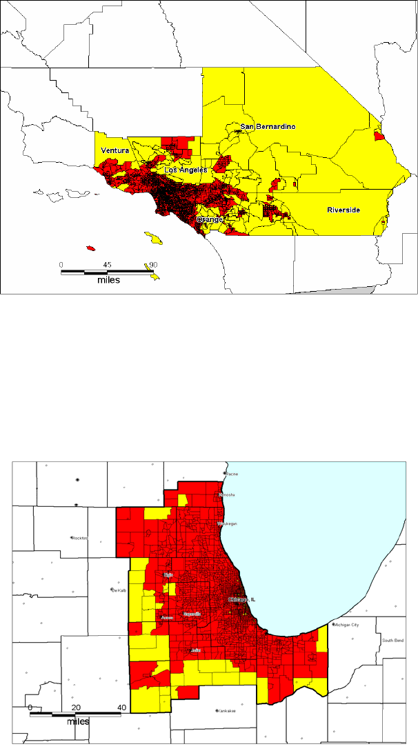
type B tracts. Figures 1 and 2 show the Los Angeles MSA and the Chicago MSA with type A tracts (dark) and type B tracts (pale);

these are category 1 MSAs. Figures 3 and 4 show two category 2 MSAs: the Champaign/Urbana category 2 MSA in Illinois (Figure 3),

and the Worcester category 2 MSA in Massachussetts (Figure 4).

Cost and timeliness are two major concerns in sample design. Consider the two extreme situations. In case I, a high quality

list of addresses/HUs exists for every area unit in the population; in case II, there are no address lists. In case II, the sample of areas

must be designed and selected well in advance of the survey to leave time for field listing of HUs in the selected areas. In case I, the

The UAU is the unit used at the final stage of selection involving areas for each part of the population. Beyond this stage, the

sampling unit is the housing unit (HU).

See O’Muircheartaigh, Colm, Stephanie Eckman, Ned English, and Catherine Haggerty,(2004)“Sampling for Inner-City Face-

to-Face Surveys” 2003Proceedings of the Section on Survey Research Methods of the American Statistical Association and

O’Muircheartaigh, Colm, Stephanie Eckman, and Charlene Weiss (2003) “Traditional and Enhanced Field Listing for Probability

Sampling” 2002 Proceedings of the Section on Survey Research Methods of the American Statistical Association.

Type A tracts are tracts in which at least 95% of the housing units (HUs) are in blocks designated with TEA code 1 – suitable

for mail-out/mail-back data collection in Census 2000.

2103

Appendix A

sample of areas can be selected very close to the time of the survey fieldwork. The cost of listing in case II will be very large, making

it impossible for many projects to support it; as a result the cost of listing will need to be amortized over a number of projects,

implying that the design of the sample of areas must be sufficiently general to be appropriate for a wide range of surveys. The design

can thus not be tailored to the particular survey. In those terms the US population frame is a mixture. For part of the population there

is a list frame; for the rest, there is not. And the two parts are intermingled in a complex way.

The design solution is to partition the frame into two parts, in one of which HUs/addresses can be selected directly from the

list; in the second part field listing must be carried out in the selected sample areas. The distinctive feature of the design is that the

two parts are not constructed from spatially connected areas, thereby giving the frame a somewhat mottled appearance.

For category 1 type MSAs, type A tracts dominate. The design solution for category 1 is to remove the type B tracts from the

category 1 MSAs. Stratum 1 is defined as those parts of category 1 MSAs that consist of type A tracts. Stratum 1 includes more than

90% of the population of category 1, but less than 50% of the area. The residual areas are treated separately (see discussion of stratum

3.2 below).

The composition of MSAs in category 2 is less extreme, in that there is a more even distribution of type A and type B tracts.

Consider again figure 3, Urbana/Champaign. This MSA is divided into two NFAs. The first consists of the areas centered on Urban

and Champaign, shaded dark in the figure. These are the type A tracts in the MSA. The pale tracts constitute a separate NFA. Stratum

2 is defined as the set of type A NFAs from category 2 MSAs; the dark areas in Figures 3 and 4 are examples. These stratum 2 NFAs

include 75% of the population of category 2, but only 20% of the area.

In category 3, the problem arises in reverse; though the dominant type of tract is type B, there are type A tracts interspersed

among them. However, though category 3 NFAs also contain both type A and type B tracts, the size of these MSA/counties is

insufficient to warrant subdivision.

Stratum 3 comprises those parts of the population where in general the USPS address list is inadequate for use as a sampling

frame. This stratum has two substrata. Stratum 3.1 contains, as NFAs: (i) the type B parts of category 2 MSAs – thus, for example, the

type B tracts in Champagin/Urbana constitute an NFA; and (ii) the category 3 NFAs. These are the primary sampling units for

stratum 3.1. Once the PSUs have been selected, segments are constructed within the selected NFAs as they have been for previous

national samples, and a field listing is carried out in the selected segments.

Stratum 3.2 comprises the type B tracts in category 1 NFAs. The pale areas in figures 1 and 2 are examples of stratum 3.2

areas. All of these NFAs appear with certainty in the sample, and fieldwork will be conducted throughout these NFAs. Consequently

it is not necessary to introduce an extra stage of sampling for this part of the population. In stratum 3.2, segments are selected directly

into the sample, and field listing is carried out as with the stratum 3.1 segments. Thus, the PSU in stratum 3.2 is the segment. See

Table A.4.

The important changes from previous GSS designs are:

• A new list-assisted sampling frame has been constructed for 72% of the population; this frame will permit re-design and re-

targeting of the sample for each successive GSS. While the same sample design, and the same selected area sampling units,

can be kept for 2006 and beyond, the design and selection could be revisited for each successive GSS without major cost

implications. Stratification and measures of size, for instance, could be adjusted based on information from the American

Community Survey.

• The size of the certainty stratum (the proportion of the population covered by certainty area selections) has been increased.

Almost half (45%) of the HUs in the population are now included in this stratum.

• Within the certainty stratum, new primary sampling units (PSUs) are being used. The PSU is now the tract (for the list-

assisted part of the population). Tracts contain about 1000-2000 HUs and therefore can be expected to have considerably

lower intracluster correlation coefficients (ρ) than the blocks/block groups (minimum size 75 HUs) that were used for

previous designs.

• In the second “urban” stratum, the new secondary sampling units (SSUs) are tracts rather than blocks/block groups; this

should lead to similar efficiency gains to those indicated above for the certainty stratum.

• In the “rural” stratum, the minimum size of SSU has been increased from 75 to 300 HUs; this should lead to smaller

intracluster correlation coefficients, ρ.

2104

Appendix A

Table A.4: Sample design for the GSS 2006 sample

Stratum % of

popn.

Description Primary (area)

sampling unit

(PSU)

Secondary (area)

sampling unit

(SSU)

Final stage

1 42% All type A tracts in

category 1 areas

Tract No 2

area stage Housing units

(HUs) from list

frame within

tract.

2 30% All type A tracts in

category 2 areas

MSA/county

[part]

Tract HUs from list

frame within

tract.

3.1 25% All counties not in

category 1 or 2; all

remaining tracts in

category 2 areas

County

[all or part]

Segment HUs from

NORC-listed

master sample

within selected

segments

3.2 3% Type B tracts in

category 1 areas

Segment No 2

area stage HUs from

NORC-listed

master sample

within selected

segments

Table A.5 gives the numbers of PSUs, SSUs, and UAUs selected within each major stratum.

Table A.5: Numbers of area units by stratum

Stratum No. of NFAs No. of PSUs No.of

SSUs

UAUs No. of

UAUs

1 24

168 (tracts) n.a. Tracts 168

2 30

30 (part MSAs/ counties) 120

(tracts)

Tracts 120

3.1

25 (part counties/MSAs)

112

(segment)

Segments 100

3.2

12 n.a Segments 12

Total

235 n.a. -- 400

90% of the population of these 24 NFAs is in stratum 1

These NFAs consist of the type A tracts in 30 MSAs

These NFAs are either whole counties/MSAs with few street-style addresses or the type B tracts from MSAs/counties

comprising stratum 2

This stratum contains the non-type A tracts in stratum 1 NFAs; they make up 6% of the population in those NFAs.

The 24 NFAs in strata 1 and 3.2 are the same areas and thus the total number of NFAs is 79.

2105

Appendix A

Figure 1: The Los Angeles MSA

Figure 2: The Chicago MSA

2106

Appendix A

Figure 3: The Urbana/Champaign MSA

Figure 4: The Worcester MSA

2107

Appendix A

NON-RESPONSIVE SUB-SAMPLING

The basic concept is to subsample the nonrespondents, adjusting the weights to keep the design unbiased. The subsample is

weighted up to represent all nonrespondents as of the cutoff date. Subsampling allows the focusing of resources on a smaller set of the

difficult cases for further attempts, thereby potentially reducing both response error and nonreponse bias.

The subsampling of nonrespondents constitutes a two-phase design, or a double-sampling scheme, that was first introduced

by Hansen and Hurwitz in 1946.

The subsampling of nonrespondents has been used in many other surveys, such as the Census

Bureau’s American Community Survey and the Urban Institute’s 1999 and 2002 National Survey of America’s Families. At NORC,

the double-sampling scheme has been used for the Chicago Health and Social Life Survey.

The typical pattern for area probability studies, such as GSS, is for a small percentage of the difficult cases to absorb much of

the resources, especially near the end of the data collection period. Increasing the initial sample size boosts the number of less

difficult cases available from the start. After the first pass, the remaining cases – those that are so much more difficult to complete are

subsampled. Considerable time and effort is spent on the subsampled cases, but since there are fewer of them, the overall field effort is

reduced.

For the 2004 GSS at the end of the preliminary field period for release 1 after about ten weeks, there were 1440 out-of-scope

cases (not housing units, vacant, etc.), 2162 completed cases, 143 partial cases and appointments, 144 final nonrespondents, and 2171

temporary nonrespondents. The temporary nonrespondents were sampled at 50% and 1086 were retained in the study and 1085 were

eliminated. The retained sub-sample cases and the partial/appointment cases were then pursued for approximately another 10 weeks.

Ulimately 2812 cases were obtained.

For the 2006 GSS at the end of the preliminary field period for release 1 after about eleven weeks, there were 1480 out-of-

scope cases (not housing units, vacant, etc.), 3418 completed cases, 283 partial cases and appointments, 259 final nonrespondents, and

4209 temporary nonrespondents. The temporary nonrespondents were sampled at 45% and 2068 were retained in the study and 2141

were eliminated. The retained sub-sample cases and the partial/appointment cases were then pursued for approximately another 10

weeks. Ulimately 4510 cases were obtained.

Since temporary nonrespondents were subsampled at 50%, they must essentially be given a weight of 2 to make the sample

representative. The weights that must be used for the 2004 GSS are discussed below in the section on Weighting. In addition, the

subsampling of nonrespondents also means that weighted figures must be used in calculating the response and other outcome rates.

The procedure utilized is discussed in Standard Definitions: Final Disposition of Case Codes and Outcome Rates for Surveys

. Lenexa,

KS: American Association for Public Opinion Research, 2004. Also available at www.aapor.org

WEIGHTING

The GSS contains three weight variables (ADULTS, OVERSAMP, FORMWT) that users should use as needed as well as

weight-related variables (ISSP+PHASE). This section briefly discusses these variables.

ADULTS

The full-probability GSS samples used since 1975 are designed to give each household an equal probability of inclusion in

the sample. (Call this probability Ph.) Thus for household-level variables, the GSS sample is self- weighting. In those households

which are selected, selection procedures within the household give each eligible individual equal probability of being interviewed. In

a household with n eligible respondents, each has probability Ph of being in a selected household, and 1/n * Ph of actually being

interviewed. Persons living in large households are less likely to be interviewed, because one and only one interview is completed at

each preselected household. The simplest way to compensate would be to weight each interview proportionally to n, the number of

eligible respondents in the household where the interview was conducted. N is the number of persons over 18 (ADULTS) in the

household. A discussion of the weight as well and a post-stratification variant of weighting by ADULTS appears in GSS

Methodological Report No. 3.

OVERSAMP

Marcus Hansen and W. Hurwitz, "The Problem of Non-response in Sample Surveys," Journal of the American Statistical

Association, 41 (Dec., 1946), 517-529.

C. Bruce Stephenson, "Weighting the General Social Surveys for Bias Related to Household Size," GSS Technical Report No. 3,

Chicago: NORC, February, 1978.

2108

Appendix A

As described in the previous section, the 1982 survey included an oversample of blacks. To make the 1982 survey a

representative cross-section, the user can either exclude the black oversample cases by excluding codes 4 and 5 on SAMPLE or

weight the file by OVERSAMP. To make the 1987 survey a representative cross-section the user can either exclude the black

oversample by excluding code 7 on SAMPLE or weight the file by OVERSAMP. Users should adopt one of these procedures in all

cases except when analyzing only blacks from the 1982 and/or 1987 cross-sections and oversamples.

FORMWT

Problems with form randomization procedures on the 1978, 1980, 1982-1985 surveys necessitate the use of FORMWT when

variables appearing on only one form are analyzed. A complete list of form-related variables appears in Appendix P. Full details on

the form randomization problem and of the weight created to correct for it appear in GSS Methodological Report No. 36.

ISSP

The International Social Survey Program supplement was administered to Form 1 cases in 1985 and as such must be

weighted for FORMWT as discussed above. In addition because this was a self-administered supplement completed after the main

GSS questionnaire there is supplement non-response. Users may wish to use the variable ISSP to study supplement non-response bias

and perhaps develop a weight to compensate for same.

POST-STRATIFICATION

In general, the GSS samples closely resemble distributions reported in the Census and other authoritative sources. Because

of survey non-response, sampling variation, and various other factors the GSS sample does deviate from known population figures for

some variables. The GSS does not calculate any post-stratification weights to adjust for such differences. For relevant discussion of

distributional variation caused by non-response and other factors see GSS Methodological Reports No. 3, 5, 9, 16, 21, 25, 79.

Differences from the Census and other changes in distributions due to alterations in sampling include the following:

1. In 1972 blacks were over-represented. The 1972 survey was the last to utilize the 1960 NORC sample frame and it

is believed to have under covered rapidly growing suburban areas.

2. All full-probability samples under-represent males. This is discussed in GSS Methodological Report No. 9.

3. Block quota samples under-represented men in full-time employment, see GSS Methodological Report No. 7.

4. Coverage of Mormons increased significantly when the 1980 sample frame was adopted. This was due to the

addition of a primary sampling unit in Utah. For more details see GSS Methodological Report No. 43.

5. People eighteen years old appear to be under-sampled although this is actually not the case. Age is assigned based

on year of birth and the assumption that one's birthday has already occurred. However, to be in the sample one must

have actually reached his/her eighteenth birthday and since the GSS is fielded in March every year only about

one-quarter of those born eighteen years prior to the current year have reached majority by the interview dates.

Thus nineteen year olds as classified on the GSS consist of approximately one-quarter who have turned nineteen

since the first of the year and three-quarters who will turn nineteen by the end of the calendar year. The same is true

Tom W. Smith and Bruce L. Peterson, "Problems in Form Randomization on the General Social Surveys," July, 1986.

See Tom W. Smith, "Attrition and Bias on the International Social Survey Program Supplement," GSS Methodological Report

No. 42, February, 1986.

C. Bruce Stephenson, "Probability with Quotas: An Experiment," GSS Methodological Report No. 3, April, 1979; Tom W. Smith,

"Response Rates on the 1975-1978 General Social Surveys with Comparisons to the Omnibus Surveys of the Survey Research Center,

1972-1976," GSS Methodological Report No. 5, June, 1968; Tom W. Smith, "Sex and the GSS: Nonresponse Differences," GSS

Methodological Report No. 9, August, 1979; Tom W. Smith, "The Hidden 25%: An Analysis of Nonresponse on the 1980 General

Social Survey," GSS Methodological Report No. 16, May, 1981; Tom W. Smith, "Using Temporary Refusers to Estimate

Nonresponse Bias," GSS Methodological Report No. 21, February, 1983; Tom W. Smith, "Discrepancies in Past Presidential Vote,"

GSS Methodological Report No. 25, July, 1982; and Tom W. Smith, "Notes on John Brehm, The Phantom Respondent: Opinion

Surveys and Political Representation." GSS Methodological Report No. 79, 1993.

2109

Appendix A

for ages 20 and up. For eighteen year olds on the GSS only those who have turned eighteen since the first of the

year are included. Thus the number of eighteen year olds in the GSS is approximately one-quarter the number of

nineteen year olds (See Appendix E). The "missing" eighteen year olds are not under-represented in the sample, but

are merely counted as nineteen year olds.

Weights for 2004-06 GSS

Due to the adoption of the non-respondent, sub-sampling design described above, a weight must be employed when using the

2004-06 GSSs. One possibility is to use the variable PHASE and weight by it so that the sub-sampled cases were properly represented.

If one wanted to maintain the original sample size, one would weight by PHASE*0.86258 in 2004 and PHASE*.80853 in 2006. This

weight would only apply to 2004-06 and would not take into account the number of adults weight discussed above. As such, it would

be appropriate for generalizing to households and not to adults. A second possibility is to use the variable WTSS. This variable takes

into consideration a) the sub-sampling of non-respondents, and b) the number of adults in the household. It also essentially maintains

the original sample size. In years prior to 2004+ a one is assigned to all cases so they are effectively unweighted. To adjust for number

of adults in years prior to 2004, a number of adults weight would need to be utilized as described above. WTSSALL takes WTSS and

applies an adult weight to years before 2004. A third possibility is to use the variable WTSSNR. It is similar to WTSS, but adds in an

area non-response adjustment. Thus, this variable takes into consideration a) the sub-sampling of non-respondents, b) the number of

adults in the household, and c) differential non-response across areas. It also essentially maintains the original sample size. As with

WTSS, WTSSNR has a value of one assigned to all pre-2004 cases and as such they are effectively unweighted. Number of adults

can be utilized to make this adjustment for years prior to 2004, but no area non-response adujustment is possible prior to 2004. Details

on the construction of WTSS and WTSSNR follow:

WTSS:

W0: Within each NFA, we calculate a probability of selection, n/N. W0 is the reciprocal of this probability of selection (N/n). At

this point, each observation stands in for a given number of cases in the frame. Because the secondary sample release was

only in the urban NFAs, cases in urban NFAs have a slightly higher probability of selection, and thus a slightly lower

baseweight, than cases in the urban NFAs.

∑W0 = frame size

W1: At the end of Phase I of data collection, we subsampled the non-responding cases with a sampling fraction f=.5. W1 for the

selected non-responding cases is then WO*(1/.5) in 2004 or for 2006 is WO*(1/.45). W1 is missing for the unselected non-

responding cases. W1=W0 for cases which were not subsampled.

∑W1 = frame size

W2: Next, we adjust the baseweight for eligibility. Not all cases in the frame are truly eligible for the survey: some addresses in

our frame are businesses, do not exist or are unoccupied. We use the eligibility rate of the sampled cases to estimate the

eligibility rate for the frame. We calculate the eligibility rate at the NFA level.

This adjustment sets the weights of the ineligible cases to missing. Cases whose eligibility could not be determined are given

fractional eligibility equal to be eligibility rate for their NFA.

Now the sum of the weights is the estimated number of eligible cases (or occupied housing units) in the frame.

∑W2 = estimated eligible cases in the frame < ∑W1

We then rescale W3 so that the sum is the total number of completed interviews. This adjustment helps prevent errors that

can arise in SPSS and in some procedures in SAS where the sum of the weights in assumed to be equal to the sample size.

The relative weights are unchanged by this adjustment.

∑ WEIGHT = number of completed interviews

WTSSNR:

W2NR: We next adjust for non-response. Weights for responding cases increase by the reciprocal of the response rate, calculated at

the NFA level. The responding cases take on the additional weight of the non-responding cases. W2NR is missing for the

non-response cases. The sum of the weights is the same as the previous step: the estimated number of eligible cases in the

frame.

∑ W2NR = ∑W2 = estimated eligible cases in the frame

W3: To account for the random selection of an adult respondent, this weight is the household-level weight (W2) multiplied by t

number of adults in the household. The sum of the weights in this step is the total number of adults in all eligible households

in the frame.

∑ W3 = estimated adults in eligible cases in the frame > ∑W2

W3NR: To account for the random selection of an adult respondent, this weight is the non-response adjusted household-level weight

2110

Appendix A

(W2NR) multiplied by the number of adults in the household. The sum of the weights in this step is the total number of adults

in all eligible households in the frame.

∑ W3NR = estimated adults in eligible cases in the frame > ∑W2NR

∑ W3NR = ∑W3

WEIGHT: We then rescale W3 so that the sum is the total number of completed interviews. This adjustment helps prevent errors that

arise in SPSS and in some procedures in SAS where the sum of the weights is assumed to be equal to the sample size. The

relative weights are unchanged by this adjustment.

∑ WEIGHT = number of completed interviews.

WEIGHTNR: We also rescale W3NR so that the sum is the total number of completed interviews. This adjustment helps prevent

errors that can arise in SPSS and in some procedures in SAS where the sum of the weights is assumed to be equal to

the sample size. The relative weights are unchanged by this adjustment.

∑ WEIGHTNR = number of completed interviews

TIME

If the merged GSS is thought of as designed to equally sample time, there are numerous deviations due to such factors as 1)

sample size variation across surveys, 2) the absence of surveys in 1979, 1981, 1992, and in odd years after 1993, 3) experiments (See

Appendix O), 4) switching of items from permanent to rotating status, 5) switching from across-survey rotation to sub-sample rotation,

6) late starting and terminated time series, or 7) some combination of these. For more information on these issues and possible

adjustments see GSS Methodological Report No. 52.

Tom W. Smith, "Rotation Designs of the GSS," Chicago: NORC, February, 1988.

2111

Appendix A Appendix A

Table A.6

NON‑RESPONSE RATES ON THE 1975‑2006 GENERAL SOCIAL SURVEYS

(Full Probability Samples Only)

Dispostion of Cases Surveys

1975 1976 1977 1978 1980 1982 1982B 1983 1984 1985 1986 1987 1987B 1988

A. Original Sample 1102 1113 2317 2344 2210 2221 2900 2222 2157 2201 2192 2250 4750 2250

B. -Out of Sample 11 16 0 20 1 0

2258

30000

3916

C. -Not a Dwelling Unit 43 126 93 130 117 84 77 45 73 77 106 78

116 219

D. -Vacant 74 217 190 197 245 172 197 227 176 206 328 261

E. -Language Problem 27 33 54 59 46 46 6 31 52 28 49 43 0 52

F. +New Dwelling Unit 24

44 79 102 97 129 77 82 42 47 50 21 42 57

G. Net Sample 972 991 1999 2084 1933 1942 494 2014 1873 1948 1944 1945 442 1916

H. Completed Cases 735 744 1530 1532 1468 1506 354 1599 1473 1534 1470 1466 353 1481

I. Refusals 162 339

206 417 309 297 66 320 320 344 365 358 57 359

J. Break-offs 2 7

K. No one Home to 22 54 48 30 41 17 23 22 46 5 19

Complete Screener 56 49

L. R Unavailable Entire 13 26 22 38 23 18 8 13 20 3 7

Field Period 41

M. Ill 12 21 37

43 75 18 60 31 39 74 55 24 50

N. Other 26

____ ___ 44 51 ___ ___ ___ ___ ___ ___ ___ ___

G. Net Sample 972 991 1999 2084 1933 1942 494 2014 1873 1948 1944 1945 442 1916

Eligibility Rate (G/A) 0.882 0.890 0.863 0.889 0.875 0.874 0.170 0.906 0.868 0.885 0.887 0.864 0.093 0.852

Reponse Rate (H/G)

0.756 0.751 0.765 0.735 0.759 0.775 0.717 0.794 0.786 0.787 0.756 0.754 0.799 0.773

Refusal Rate (I+J/G)

0.169 0.208 0.173 0.200 0.160 0.153 0.134 0.159 0.171 0.177 0.188 0.184 0.129 0.187

Unavailable Rate (K+L/G)

0.036 -- 0.040 0.034 0.035 0.033 0.113 0.017 0.026 0.016 0.018 0.034 0.018 0.014

Other Rate (M+N/G)

0.039 -- 0.022 0.031 0.046 0.039 0.036 0.030 0.017 0.02 0.038 0.028 0.054 0.026

Includes screened households with no Blacks.

This corresponds to RR5 (response rate 5) in the American Association for Public Opinion Research's Standard Definitions of the

Final Dispositions of Case Codes and Outcome Rates for RDD Telephone Surveys and In-Person Household Surveys (2006).

In 2004+ the rate is a weighted response rate as provided in AAPOR (2006). The case figures in the 2004+ columns do not yield the

calculated rates because they are unweighted. Also, see Appendix A, "Non-response sub-sampling" on the sub-sampling on non-respondents in 2004+

Refusal rate 3 in AAPOR's Standards.

2112

Appendix A Appendix A

Table A.6 (Continued)

NON‑RESPONSE RATES ON THE 1975‑2006 GENERAL SOCIAL SURVEYS

(Full Probability Samples Only)

Dispostion of Cases Surveys

1989 1990 1991 1993 1994 1996 1998 2000 2002 2004 2006

A. Orig

2250 2165 2312 2296 4559 4559 4567 4883 4890 6260 9535

B. -Out 20000100000

C. -Not 57 70 85 65 103 158 158 242 152 638 392

D. -Vac

212 232 256 246 524 493 573 531 622 608 1058

E. -Lan

72 47 67 66 143 136 146 178 209 301 139

F. +New 74

41 46 31 57 43 55 94 36 0 41

G. Net

1981 1857 1950 1950 3846 3814 3745 4026 3943 4713 7987

H. Comp

1537 1372 1517 1606 2992 2904 2832 2817 2765 2812 4510

I. Refusals

346 355 323 285 708 757 755 1044 1031 621 987

J. Break-offs

K. No o

26 61

Complete Screener 54 18 18 60 66 97 59 65 48

L. R Unavailable Entire

Fiel

815

M. Ill

59 54 56 41 128 93 92 68- 88- 130 185

. Othe

___ ___ ___ ___ ___ ___ ___ ___ ___ ___ ___

G. Net

1981 1857 1950 1950 3846 3814 3745 4026 3943 3628 4510

Eligibi

0.884 0.858 0.843 0.849 0.844 0.837 0.820 0.824 0.806 0.753 0.838

Respons

0.776 0.739 0.778 0.824 0.778 0.761 0.756 0.700 0.701 0.704 0.712

Refusal 0.175 0.191 0.166 0.146 0.184 0.198 0.202 0.259 0.261 0.225 0.233

Unavail

0.017 0.041 0.028 0.009 0.005 0.016 0.018 0.024 0.015 0.024 0.011

Other R

0.030 0.029 0.029 0.021 0.033 0.024 0.025 0.017 0.022 0.047 0.044

2113

Appendix B

APPENDIX B:

FIELD WORK AND INTERVIEWER SPECIFICATIONS

1972-2000

This study employed standard field procedures for national surveys, including interviewer hiring and training by area supervisors in

interviewing locations when necessary. The sampling procedures were reviewed by having interviewers take a training quiz after they

had studied the sampling instructions specific to this study (see Appendix A for a discussion of the sample). Around the same time,

publicity materials were sent to area supervisors; these included letters to be mailed locally to the Chief of Police, the Better Business

Bureau, the Chamber of Commerce, and the various news media.

After these steps were completed, interviewers received materials needed for data collection (assignments, specifications, blank

interview schedules). Each interviewer completed one practice interview which was evaluated at NORC. Actual interviewing then

commenced; completed interviews were immediately returned to NORC where they were edited for completeness and accuracy.

Twenty percent of the interviews were validated. Feedback on specific problems was given to individual interviewers and on general

problems to all interviewers.

Once field work was completed, the edited questionnaires were coded and keypunched, and the resulting data were cleaned (see

Appendix C: General Coding Instructions).

The following section contains the interviewer specifications in one continuous listing. Originally, the specifications were com-

municated to interviewers by means of an annotated interview schedule and memoranda on specific interviewing problems. The

specifications inform the interviewers of the intent of the question, provide caution signals where a potential problem may exist, and

recommend probes or provide interpretations which can be suggested to the respondent should the respondent have difficulty in under-

standing the question. All the specifications work toward increasing the internal validity of the data collected.

Questions which had no specifications are not included in this section. If a specification or explanation modifies an entire ques-

tion, the question is not repeated here. If a specification modifies one response category, or only one section of the question, the

modified portion is repeated here and appears in brackets "[ ]."

Specifications from the most recent survey are given first. Earlier specifications are given next. Notes about additions, omissions,

etc. refer to the immediately preceding entry. "None" means that no specification was used that year. Questions not listed below have

never had specifications.

2002+

In 2002 the GSS switched to computer assisted Personal Interviewing (CAPI). There are no printed questionnaires, but the show-

cards are still printed. Manual edits and keypunching are eliminated. Training now includes learning how to operate CAPI. Data

validation and cleaning remains similar to pre-CAPI procedures described above.

2114