Analysis of Sequencing and Scheduling Methods for Arrival Traffic

NASA Technical Memorandum 102795 _.--------_,,

Analysis of Sequencing and

Scheduling Methods

for Arrival Traffic

Frank Neuman and Heinz Erzberger

April 1990

k ::_ ,i,-i' ..... "; i 'i. _

NASA

National Aeronautics and

Space Administration

NASA Technical Memorandum 102795

Analysis of Sequencing and

Scheduling Methods

for Arrival Traffic

Frank Neuman and Heinz Erzberger, Ames Research Center, Moffett Field, California

April 1990

N/LSA

National Aeronauticsand

SpaceAdministration

Ames Research Center

Moffett Field, California 94035-1000

SUMMARY

The air traffic control subsystem that performs scheduling is discussed. The function of the

scheduling algorithms is to plan automatically the most efficient landing order and to assign optimally

spaced landing times to all arrivals. Several important scheduling algorithms are described and the

statistical performance of the scheduling algorithms is examined. Scheduling brings order to an arrival

sequence for aircraft. First-come-fin'st-served scheduling (FCFS) establishes a fair order, based on

estimated times of arrival, and determines proper separations. Because of the randomness of the traffic,

gaps will remain in the scheduled sequence of aircraft. These gaps are filled, or partially tidied, by time-

advancing the leading aircraft after a gap while still preserving the FCFS order. Tightly scheduled

groups of aircraft remain with a mix of heavy and large aircraft. Separation requirements differ for dif-

ferent types of aircraft trailing each other. Advantage is taken of this fact through mild reordering of the

traffic, thus shortening the groups and reducing average delays. Actual delays for different samples with

the same statistical parameters vary widely, especially for heavy traffic.

ABBREVIATIONS

ARTCC Air Route Traffic Control Center (also called Center)

ATC air traffic control

CPS

constrained position-shift optimization scheduling method

ERM en route metering

ETA

estimated time of arrival at the runway (no interference from other aircraft)

FAA Federal Aviation Administration

FCFS first-come-first-served scheduling method

N traffic density = demand = number of aircraft/hr wanting to land

STA

scheduled time of arrival at the runway (includes required delays)

TA time-advance optimization scheduling method

TMA Traffic Management Advisor

INTRODUCTION

An automated system for air traffic control (ATC) may be divided into three principal subsystems

whose functions involve sensing, planning, and controlling. The subject of this report is the planning

subsystem that performs scheduling. The function of the scheduling algorithms is to plan automatically

the most efficient landing order and to assign optimally spaced landing times to all arrivals. Several

important scheduling algorithms are first described, and the statistical performance of the scheduling

algorithms is then examined.

The most straightforward scheduling method assigns the landing order on a first-come first-served

basis (FCFS). In this method, after aircraft enter the Air Route Traffic Control center (ARTCC), they are

scheduled in the order in which they are predicted to land, using a nominal path, flight plan, preferred

descent speeds, and altitude profiles. The FCFS scheduler adds appropriate delay times to insure proper

spacing, which depends on the weight classes of the aircraft.

FCFS scheduling can be compared with present technology. An operational scheduling system used

at some ARTCCs is called En Route Metering (ERM). ERM generates rough approximations for the

estimated times of arrival (ETAs) and bases the FCFS ordered scheduled times of arrival (STAs) on

those ETAs. The main use of ERM is to provide a specified flow rate from the Center to the TRACON.

It does not perform optimization of schedules, nor does it provide advisories to achieve accurate arrival

times. Also, the order assigned by the current scheduler is often not followed; rather, it is used primarily

to indicate landing-slot availability to which the controller may assign any aircraft. Current scheduling

and metering does not use spacing depending on the weight classes of aircraft; instead, it uses the same

time-interval between all types of aircraft. However, the time-interval can be changed by the operator to

produce a specified landing rate.

An effective method of reducing the average delay time without changing the order of the aircraft is

called time-advance (TA). In this his method, the beneficial effect of occasionally speeding up an air-

craft during periods of heavy traffic in order to reduce gaps that naturally occur in FCFS schedules is

recognized. It is called time-advance herein and in reference 1 and is called the negative delay effect in

references 2 and 3.

The spacing requirements mentioned earlier offer the opportunity to optimize the landing sequence,

thereby improving on the FCFS and TA methods by minimizing the average delay per aircraft. A

sequencing and scheduling optimizing method called constrained position shift (CPS) was developed

several years ago by Dear (ref. 4). The CPS method assumes that an initial landing order has been

determined by FCFS and that all aircraft are tightly packed, that is, that they have minimum time-

separations. By rearranging the landing order, while not shifting any aircraft from its original position in

the sequence by more than a few places, the total time between the first aircraft and the last aircraft can

often be reduced. Though CPS is conceptually straightforward, its implementation in a real-time algo-

rithm is more complex because of bunching and of gaps in the arrival sequence. The gaps are due to the

randomness of the arrival times of aircraft in the terminal area. CPS must, therefore, be applied to indi-

vidual groups of aircraft as we have done here, or the algorithm's performance index must be rewritten

from that given in appendix A, so that it minimizes the sum of the scheduled flight times instead.

Anothermethodof optimization,thebranch-and-boundtechnique,wasusedin anATC advisory

systemcalledCOMPAS(ref. 5).Bothoptimizationmethods,CPSandbranch-and-boundattemptto

sequenceincomingaircraftin suchamannerasto minimizethetotal delayfor all aircraft,andfor both

methodsvariousrestrictionsapplyin ordertoobtainfeasiblesolutions.

Threeof thesemethodsof scheduling,FCFS, TA, and CPS have been implemented in a Traffic

Management Advisor (TMA) Station, which is part of an automated system for the management of

arrival traffic (ref. 1). The scheduler in this system permits the selective use of any of these scheduling

schemes, and it contains other features that are important for the human interaction with the automated

scheduler.

The purpose of this report is to statistically evaluate the scheduling methods that are implemented in

the TMA. This is done using a large number of realistic traffic samples to determine their overall effect

on aircraft delays. Additionally, the analysis is used to show the effects of other variables on delays such

as traffic distributions, lengths of traffic samples, and winds. Also, analysis of the results for an optimal

single-position-shift CPS, which cannot be implemented in an operational ATC system, permits the

design of a heuristic CPS that can be implemented.

First, we discuss three scheduling algorithms, FCFS, TA, and CPS, wherein each successive algo-

rithm improves on the preceding one by further reducing the average delay for all aircraft. Then, we

build a model of incoming traffic to a hub airport for the purpose of evaluating the scheduling algo-

rithms. Finally, we generate a sufficiently large number of randomly chosen traffic samples to obtain the

statistical characteristics of the scheduling algorithm as a function of mix of aircraft and traffic density.

The primary criterion of performance is average delay per aircraft. In addition, we will examine a few

individual traffic samples, to determine where scheduling algorithms may be simplified or improved.

An exact solution of the constrained position-shift problem is presented in appendix A, which was

written by Jeffrey C. Jackson (School of Computer Science, Carnegie-Mellon University, Pittsburgh,

PA). The combined FCFS and time-advance algorithm is given in appendix B.

SCHEDULING ALGORITHMS

In order to schedule aircraft for landing at an airport in an efficient manner one has to know the sepa-

ration requirements for different types of aircraft. We will therefore discuss these requirements before

going to the actual scheduling algorithms.

Separation Requirements

Separation requirements are an essential input for all types of scheduling algorithms. As stated

earlier, we are dealing with two types of aircraft, heavy and large. For each type, the Federal Aviation

Administration (FAA) specifies a separation distance at landing that is dependent on the sequence

heavy-heavy, heavy-large, large-large, large-heavy. The minimum separation matrix is shown below

(separation distances are in nautical miles).

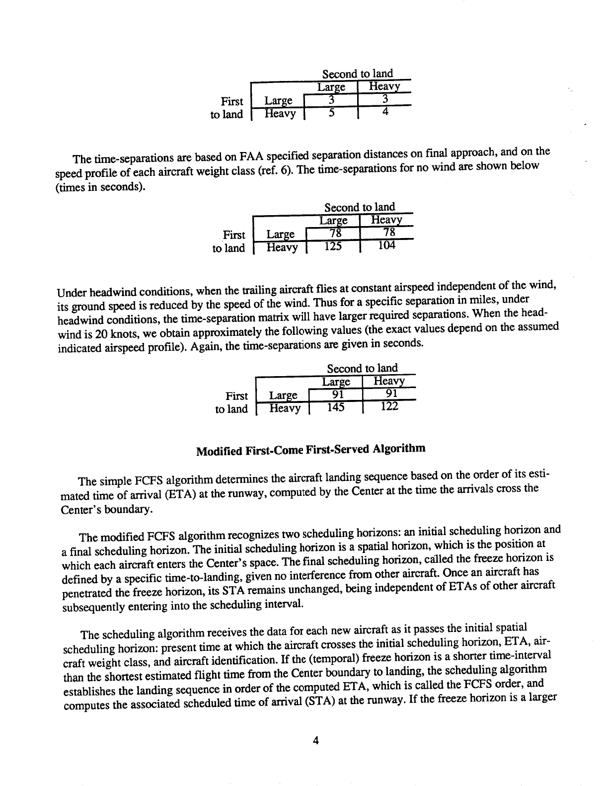
Second to land

First Large 3 3

to land Heavy 5 4

The time-separations are based on FAA specified separation distances on final approach, and on the

speed profile of each aircraft weight class (ref. 6). The time-separations for no wind are shown below

(times in seconds).

Second to land

Large [ Heav),

First Large 78

oavyl I

125

Under headwind conditions, when the trailing aircraft flies at constant airspeed independent of the wind,

its ground speed is reduced by the speed of the wind. Thus for a specific separation in miles, under

headwind conditions, the time-separation matrix will have larger required separations. When the head-

wind is 20 knots, we obtain approximately the following values (the exact values depend on the assumed

indicated airspeed profile). Again, the time-separations are given in seconds.

Second to land

First Large 91 91

to land Heavy 145 122

Modified First-Come First-Served Algorithm

The simple FCFS algorithm determines the aircraft landing sequence based on the order of its esti-

mated time of arrival (ETA) at the runway, computed by the Center at the time the arrivals cross the

Center's boundary.

The modified FCFS algorithm recognizes two scheduling horizons: an initial scheduling horizon and

a final scheduling horizon. The initial scheduling horizon is a spatial horizon, which is the position at

which each aircraft enters the Center's space. The final scheduling horizon, called the freeze horizon is

defined by a specific time-to-landing, given no interference from other aircraft. Once an aircraft has

penetrated the freeze horizon, its STA remains unchanged, being independent of ETAs of other aircraft

subsequently entering into the scheduling interval.

The scheduling algorithm receives the data for each new aircraft as it passes the initial spatial

scheduling horizon: present time at which the aircraft crosses the initial scheduling horizon, ETA, air-

craft weight class, and aircraft identification. If the (temporal) freeze horizon is a shorter time-interval

than the shortest estimated flight time from the Center boundary to landing, the scheduling algorithm

establishes the landing sequence in order of the computed ETA, which is called the FCFS order, and

computes the associated scheduled time of arrival (STA) at the runway. If the freeze horizon is a larger

time-intervalthanthe shortestestimatedflight time from the Center boundary to landing, the situation is

more complicated, as will be discussed next.

For aircraft that enter the scheduling horizon, the STAs are computed as follows. If no other previ-

ously scheduled aircraft's ETA is later than that of the newcomer's ETA, then the STAs of the earlier

scheduled aircraft are not disturbed, and the newcomer is assigned a time equal to its ETA or the time

that ensures the minimum time-separation required for the types of aircraft that are following each other,

whichever is larger. If a new arrival's ETA falls ahead of the time slots reserved for previously sched-

uled aircraft, and if none of the already scheduled aircraft had its schedule frozen, then the new arrival is

inserted ahead of these aircraft in the order of the ETA and at the proper spacing from the next earlier

aircraft. All aircraft following the new arrival are re-spaced with the proper spacing. If frozen scheduled

aircraft have STAs later than the new arrival's ETA, we first check if a sufficiently large gap exists such

that the new aircraft can be scheduled ahead of the frozen aircraft without changing any other aircraft's

position. If proper separation cannot be maintained, the new aircraft is scheduled in front of the first air-

craft whose schedule has not yet been frozen, and the non-frozen aircraft behind the newcomer are

rescheduled. (If frozen aircraft are present, this is not strictly an FCFS scheduling, even though we call it

that in this report.)

Aircraft arriving at the boundary of the initial scheduling horizon appear unevenly spaced. Therefore

the FCFS algorithm creates groups of tightly scheduled airplanes with large gaps between individual

groups. With the FCFS algorithm, the first aircraft in a group requires no delay whereas succeeding air-

craft, on the average, require increasingly larger delays.

Time-Advance Method

The TA method, which was called the negative delay effect in reference 2, operates on the first air-

craft of each group, and does not change the existing order (e.g., FCFS). The fwst aircraft in a group is

speeded up to arrive sooner than its nominal ETA, and all aircraft in the group following it will have

their delays decreased by the same amount of time. This also reduces or closes the initial intergroup gap.

Since speedup is costly, the first aircraft is speeded up only when at least the immediately following air-

craft requires a delay, which is shortened because of the speedup of the first aircraft. In this statistical

evaluation, we do not have a program that calculates maximum, minimum, and nominal ETAs from air-

craft, navigation, and weather data. In the absence of actual minimum ETA data, we chose a maximum

time-advance of 1 rain for all aircraft. In an implemented scheduling system, the time-advance for

each leading aircraft in a group can be based on a fraction of the calculated values of the available

time-advance.

When the (temporal) freeze horizon has a smaller value than the time of the shortest flightpath,

FCFS and TA applied to the incoming traffic result in the same overall aircraft order. This is not so

when the freeze horizon has a larger value than the time for the shortest flightpath. A more detailed

description of the combined FCFS and TA algorithm is given in appendix B.

Constrained Position-Shift Method

Optimal CPS- As previously mentioned, the CPS method reorders the existing FCFS order by

taking advantage of different separation requirements for different aircraft classes. Reordering makes

sense only within a group. It is theoretically most effective when the groups are long (heavy traffic).

Two aircraft are considered for reordering by a single position, provided that they arrive at the airport

from different directions. This prevents possible overtakes within a sector. An optimal single-position-

shift algorithm was developed by Jackson (unpublished) and is described in appendix A. A necessary

restriction is that none of the aircraft in the group can be given a time-advance of more than 1 rain. As

the algorithm is written, this restriction can only be tested after the algorithm has proposed position

switches. Various non-optimal methods of removing the violations to the restrictions make the overall

algorithm non-optimal. Because of computational constraints on the scheduling algorithms operating in

real-time, and because of the physical constraints of time-advancing aircraft, the use of larger position

shifts is not practical. Similar to the TA method, in a more complete simulation, one could use a time-

advance equal to a percentage of the available time-advance for the given aircraft.

Heuristic CPS- The optimal CPS is based on the dynamic programming principle, and the solution

of all position shifts is found only at the end of each group of aircraft. In an actual system, we have a

scheduling window with a time-interval often much shorter than that of a group of aircraft, especially for

heavy traffic, when CPS would be useful. As discussed in the results section, optimal CPS switches air-

craft positions in such a way as to group heavy aircraft when possible. The following groupings are

considered for the heuristic CPS, where "H" means heavy and "L" means large aircraft. Groups of

size 5 which contain LHL: LHLHH -> LLHHH, HHLHL -> HHHLL, LHLHL -> LHHLL, and one

HL or LH switch suffices. The sequence HHLHH is not switched. In addition, two longer patterns

are considered if a sufficient number of aircraft are in the scheduling window: a pattern of size 6,

LHLLHL -> LLHHLL, which requires one HL and one LH switch, and a pattern of size 7, which also

requires one LH and one IlL switch: LHLHLHL -> LLHHHLL. Two additional patterns, those that

require a two-position shift of a heavy aircraft, are also checked for: LHLLHH -> LLLHHH and

HHLLHL -> HHHLLL. This makes it possible that under certain conditions the heuristic CPS may

work better than the single-position-shift optimal CPS.

For all these patterns, the earliest aircraft can be below the freeze horizon, since it is never involved

in a switch; nevertheless, it determines which pairs of aircraft are switched. One additional pattern is

searched for at the end of each group of aircraft LHL gap L or H -> LLH gap L or H. This increases the

length of the gap. Before switching, the old order of aircraft types and STAs is preserved. After the new

STAs have been calculated, using the minimum time-separation matrix shown previously, we check to

verify that all delays STA[j] - ETA[j] are less than -1 min (time-advance of less than 1 rain). If this is

not the case, the old unswitched values are restored. This automatically takes care of larger gaps in the

original aircraft sequence. The longer patterns are checked by using the original sequence of aircraft

types, and the possible changes from matching a shorter pattern are changed to the longer pattern, pro-

vided they meet the delay criteria. As desired, attempted rescheduling over a large gap will cause the

delay criteria to fail. No performance criterion needs to be calculated, since each switch guarantees some

reduction in average aircraft delay of the traffic sample.

TRAFFIC MODEL

Toward an Accurate Traffic Model

To evaluate the scheduling algorithms for a particular situation, one needs an accurate traffic model.

Such a model might be based on scheduled airline arrivals for specific days of the week, including

planned routes and aircraft types. Such lists are available at ARTCCs and are presently used by the traf-

fic managers to predict peak traffic times. However, these lists are not accurate enough to predict aircraft

arrivals at the Center boundary, because, as will be explained next, scheduled traffic must be consider-

ably modified before it crosses the Center boundary.

All traffic samples discussed herein are based on arrivals at Denver Center. Scheduled traffic at

Denver for a particular date and time-interval is illustrated in figures 1 and 2. It can be seen from these

figures that the incoming traffic was heavily concentrated in the 30-min period from 7:45 A.M. to

8:15 A.M. (local time), and that almost all traffic was from the NE and SE. In fact, there were 56 aircraft

scheduled in a 33-min time interval. Such peaks do not get completely flattened out by the natural sta-

tistical blurring owing to random delays in takeoffs, errors caused by winds, and flight technical factors,

but the flattening process is aided by deliberate changes, such as ground holding and increases in in-trail

spacing. To get a more precise model of the traffic, one would have to collect data for many days on air-

craft crossing the Center boundary, along with aircraft type and planned route. Such data are difficult to

obtain. Therefore, we are using a somewhat less detailed model, which is based on gross traffic statistics.

Traffic Model for Studying Scheduler Effect

The purpose of this work is to describe a statistically accurate traffic model typical of peak hours at

Denver, which was used to investigate different scheduling algorithms. When many traffic samples are.

analyzed, the model provides a good insight into traffic problems resulting from the random nature of

traffic arriving at the Center boundaries, even though the traffic scheduled by the airlines may be almost

identical for many days. The aircraft arrival rates, in-trail distances, and their statistical variations are

realistic for each jet route. These arrival rates may be changed, depending on what time of day is simu-

lated. Also, traffic from one direction can be made heavier than that from the other direction. Moreover,

the model assumes that the incoming traffic on different jet routes is not coordinated for conflict avoid-

ance at the various route junctions or at touchdown. Coordination and conflict resolution have to be

accomplished in the Center sectors (with the help of the scheduler) and finally in the TRACON area.

Jet traffic arrives in Denver Center's northwest arrival sectors along four routes, and in the northeast

arrival sectors along three routes (fig. 3). The northwest traffic is handed to the TRACON through the

Drako feeder gate, and the northeast traffic through the Keann feeder gate. Incoming traffic from the

lower half-plane is not simulated, since it is landing on a separate runway during VFR operation.

One of the traffic directions usually carries high-density traffic and the other direction usually carries

low-density traffic. In our simulation, the high-density direction carries about 70% of the traffic. Any

other ratio of high-density-to-low-density traffic can be chosen. For this simulation, on the average, each

of the four routes in the Drako area carries 25% of the NW traffic, and each of the three routes in the

Keannareacarriesone third of the NE traffic. Also, on the average, of all aircraft arriving, 30% of all

traffic is heavy jets, 70% is large jets. Presently we are dealing only with two types of aircraft, heavy and

large. At Denver, small aircraft usually land on a different runway. These assumptions will sometimes

be varied to observe the effects on the delay statistics.

Actual route-traversal times within the Center boundary are shown in the following table. These

times vary considerably and make it difficult to develop a schedule that remains fixed in time, one that a

controller can use. Hence, the times for each route were approximately equalized (the "total" columns in

the table), which is equivalent in a real system to extending the shorter routes, J170, J10, and J157 into

the adjacent Centers. The total route-traversal times are not arbitrarily made equal, since in a real system

route-traversal times vary as a function of aircraft types and winds, and the scheduler must be able to

handle routes of various lengths. This simulation is limited to constant route-traversal times for each

route, independent of the type of aircraft, thus avoiding the study of possible conflicts on the same route,

when a faster aircraft may pass a slower one.

Jet route

No.

J163

J 56

J170

J24

Jl14

J10

J157

Route traversal times

Within Center

boundaries, min

42.30

45.45

28.50

47.78

41.43

25.10

34.11

Total,

min

42.30

45.45

45.00

47.78

41.43

45.00

Through

Drako

Through

Keann

Given the chosen statistical traffic parameters, such as the landing rate and the sample time-interval, the

start times and routes for exactly M aircraft are generated uniformly for the time-interval specified,

where M = (landing rate x time interval ), and is rounded to an integer. The aircraft arrival rate for each

route is chosen based on the traffic load at Denver. Since time en route varies between 42.3 and

47.78 min for different routes, the nominal landing times have been rearranged so that the rectangular

distribution for each route centers on one-half of the time-interval. This results in an overall nonuniform

distribution for start and landing times, where only the first and last few minutes are affected. The uni-

form distributions of start times for individual routes sometimes violate the minimum separation stan-

dard of 3 min on each route. Hence, the times at which the aircraft cross the original Center boundary for

each route are modified iteratively, starting from the earliest aircraft, by shifting each aircraft that vio-

lates the specified minimum in-trail spacing time-interval to a later time until all aircraft meet the speci-

fied in-nail spacing. This often generates several equally spaced aircraft, especially in heavy traffic,

which duplicates real traffic situations. Also, this modification sometimes makes the traffic sample

longer than the specified interval, especially when large in-trail spacing time-intervals are specified.

Again, this is thought to be realistic, since a scheduling time-interval for a fixed number of aircraft must

get stretched out, as the example in figures 1 and 2 showed.

To studythesensitivityof calculated delays as a function of the distribution of aircraft in the specified

time-interval, we also provide the choice of a triangular distribution of aircraft for each jet route.

RESULTS

First, individual traffic samples will be discussed to give a clear picture of the generation of traffic

samples and their statistical character, as well as to demonstrate the effect that scheduling has on delays.

Second, statistical results will be discussed in terms of cumulative probability distributions.

Time Diagrams of Traffic Samples and Associated Delays

In this section we present a variety of traffic samples. Since traffic samples in tabular form are hard

to grasp, a graphical presentation has been developed. The graphical presentation of the sample affords a

quick way of understanding the interrelations of the various time-ordered lists and of grasping causes of

delays, as well as suggesting some remedies. Using an example, we will first describe the time diagram

in detail and then present various traffic samples, limiting the discussion to major points. Figures 4(a)

and 4(b) show a theoretical traffic sample at Denver (arrival rate of 25 aircraft/hr from the NE and NW).

Given a set of parameters, such as arrival rate (demand), sample time-interval, percent of total traffic on

each route, minimum in-trail spacing, and freeze horizon, each random-number generator seed defines

one traffic sample. Knowing this seed, one can examine in detail unusual traffic sequences detected

during the statistical runs.

In all the traffic samples shown, two thirds of the traffic is through Drako and one third through

Keann. The mix of large-to-heavy aircraft is 70% to 30%. The traffic sample time-intervals are 1.5 hr,

with no traffic before or after. The minimum in-trail spacing in the Center is 3 min, which often results

in several aircraft on a route exactly 3 min apart.

The closely spaced top horizontal lines in figures 4(a) and 4(b) are time lines for each jet route. They

are from top to bottom, J157, J10, Jl14, J24, J170, J56, and J163 (see fig. 3). The dots on each horizon-

tal time line show when an aircraft is crossing the Center boundary on a given jet route. The time-scale

for these time-lines is given above the lines. The time-scale for the ETAs and STAs has been shifted by

a constant amount (40 min) to make the figure more compact. This scale is shown below the graph.

Each downward slanting line is called a scheduling line for one aircraft. The vertical top portion of

each scheduling line begins at the appropriate jet route time-line and ends at an imaginary horizontal

line, the Center boundary arrival-time-line. A slanted straight line connects the vertical line's lower end

to the ETA. This time represents the time the aircraft would arrive at the runway, if there was no inter-

ference from any other aircraft or from unknown navigation errors and environmental conditions. The

sequence of all ETAs determines the FCFS order to be preserved (at least approximately) for fair

scheduling.

Any two lines that cross between the Center boundary arrival time and the ETA belong to two air-

craft on different routes, where the aircraft on the shorter route is arriving later at the boundary, but

whose ETA is earlier than that of the other aircraft.

The horizontal component of the line between ETA and FCFS STA in figure 4(a) or the ETA and

FCFS + TA STA in figure 4(b) represent the scheduled delay to meet separation requirements. If the

scheduling line is vertical, no delay is required for the particular aircraft. The more delay the greater the

slant of the line. If none of the lines intersect, as in figure 4(a), the FCFS order has been preserved,

which is the case when the scheduling horizon is selected below the time for the shortest route. The

average delay per aircraft in minutes is shown for each scheduling method; for example, under FCFS the

average delay is 0.88 rain, and further schedule optimization reduces the average delay.

In figure 4(b), for the same arrival data, the scheduling freeze horizon was deliberately chosen larger

than the time it takes to fly most routes (45 rain), hence, lines between ETAs and (FCFS + TA) STA

sometimes intersect, showing that the FCFS order has been altered. Since FCFS and TA are not separa-

ble in their effects (the FCFS order is not preserved), only the joint schedule is shown (i.e., FCFS + TA).

Scheduling around frozen aircraft often has the effect of increasing the total delay for the traffic sample

when compared with strict FCFS scheduling, as demonstrated by comparing the average delays in fig-

ures 4(a) and 4(b), where the FCFS + TA average delay increased from 0.18 to 0.52 rain. ( In a few

samples of the several thousand analyzed, this trend was reversed in cases when changing the FCFS

order mimics an intelligent CPS.)

The straight line between FCFS time and TA time in figure 4(a) shows the effect of time-advance.

An aircraft that had zero FCFS delay is a candidate for time-advance, provided that it is the leader of a

group of at least two aircraft. The aircraft is speeded up by 1 rain or until the gap to the preceding air-

craft is reduced to the minimum allowable, whichever is the smaller time-advance. Commercial jet air-

craft have only limited capability of speeding up in the descent phase, and a maximum of l-rain time-

advance is thought to be typical. The leading aircraft incurs a fuel cost flying above its preferred speed;

All other aircraft in the group that are not speeded up beyond their ETA will benefit by having their

FCFS delay reduced by the amount of time-advance of the leading aircraft. For time-advance, none of

the aircraft scheduling lines cross, and the previous order is preserved.

The final portion of the aircraft scheduling line shows the absence or presence of CPS. Since we

allow only a single position shift, only adjacent lines cross (see figs. 4(a) and 4(b)). Only the scheduling

lines for aircraft going through Keann have a dot on the FCFS + TA line to indicate whether we consider

position switching for two aircraft from the same direction NE CKeann) or NW (Drako), with a resulting

overtake condition, which would add to controller workload. Notice that in this example, for each con-

strained position shift, one aircraft arrives from the NW, the other from NE. Thus, possible overtakes are

prevented.

The short vertical lines underneath each aircraft time line indicate the type of aircraft, a longer line

for heavy aircraft and a shorter line for large aircraft. Where the traffic is tightly bunched, it can be noted

that the separations differ, depending on the successions of types of aircraft discussed earlier.

The total number of time-advance commands to aircraft goes up for smaller numbers of aircraft per

hour, because the groups of aircraft for a 1.5-hr traffic sample become shorter and more numerous, and

each leading aircraft of a group must be time-advanced. This is illustrated for four traffic samples in

figures 5(a) to 5(d). The traffic samples are chosen for light traffic (25 aircraft/hr) and heavy traffic

(40 aircraft/hr), one sample each with relatively low average delay and the other sample with excep-

tionally large delay. Figure 5 shows what causes relatively small and large delays. We have small

average delays when the ETAs are uniformly spread over the time-interval considered and are without

large gaps, and we have large average delays when the opposite is true. We can see that for low-density

traffic or well-spread traffic, TA should not be used, since delay is small already, and the cost in time-

advance for the modest delay reduction is high, 12.16 min in figure 5(a) and 14.49 min in figure 5(c).

There are many short groups, and many aircraft would have to fly faster than their preferred speed

profiles. On the other hand, the cost in time-advance for heavy or bunched traffic is relatively small,

2.55 min in figure 5(b) and 2.22 min in figure 5(d), since only three aircraft needed to be speeded up in

both cases. Figures 5(b) and 5(c) also show the modest improvement that can be achieved when CPS is

added to TA optimization. For figures 5(a) and 5(d), CPS found no position shift that gave reduced

delays. It is difficult to determine a break-even point for TA versus no TA, since both time and fuel are

involved either as savings or as cost for all aircraft whose schedules are affected.

Figures 6(a) and 6(b) show a traffic sample in which CPS is applied with and without permitting

overtakes. In this example, two additional heavy aircraft could be grouped together with overtakes

permitted, resulting in a reduction of the average delay per aircraft from 2.87 rain to 2.72 rain.

It was shown in the Scheduling Algorithm section that a 20-knot headwind upon landing increases

the required time-separations. A traffic sample illustrates this in figure 7, for FCFS only, for both both

no wind and for a 20-knot headwind. In this example, for an identical sequence of ETAs, the average

delay for FCFS scheduling is increased from 2.31 to 4.05 rain. Therefore, winds can play a major role in

causing delays.

Figure 8 shows parts of the traffic-sample diagrams having to do with CPS only. CPS tries to reduce

the length of a group of aircraft, which reduces the average delay of all aircraft. The cost of such delay

reduction is the fuel cost for those aircraft that have to be time-advanced beyond their ETA. Therefore,

CPS shows the most benefit in reduced average delay when the position switching is done early in a

large group, thus reducing the time delay for all following aircraft in that group. Switching at the end of

a group is of little benefit in reducing the average time delay (top example of fig. 8), but controllers pre-

fer to place a heavy aircraft at the end of a group. The remainder of figure 8 shows how CPS groups the

heavy aircraft together by either time-advancing or by delaying the heavy aircraft. In this manner,

groups of two, three, or four heavies are formed. Figure 8 shows only the reduction in delay: the group

becomes shorter. The cost of such position switching depends on data not shown here; namely, whether

the aircraft that are switched toward an earlier arrival time simply have their delay reduced, or if they

have to speed up to arrive earlier than their desired time of arrival.

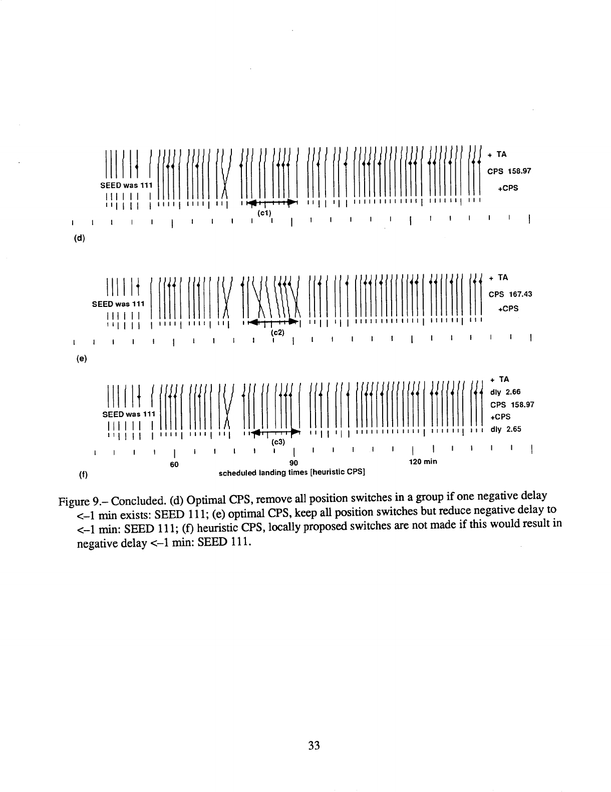
The optimal CPS algorithm assumes that a tightly scheduled group of aircraft can be reordered such

that it is again tightly scheduled with no more than the minimum required gaps. After calculating the

new order of aircraft, we find that sometimes the delay of some aircraft in the group decreases so that

they have a negative delay of less than 1 min. In such cases, two alternative choices were made to meet

the restriction (see the captions of figs. 9(a) and 9(b)). Either choice satisfies the restrictions at only a

small loss of optimality when many samples are considered. Comparing the total delays for all aircraft in

the sample of figures 9(a) and 9(b) with those of 9(d) and 9(e), we see that there is no clear choice of

methodfor meetingthemaximumnegative-delayrestriction.Tobuild thisrestrictioninto thealgorithm

directlywould unnecessarilyincreaseitscomplexity.This is notwan'anted,sincethealgorithm,asit

stands,is notusefulfor anoperationalsystem,whichhasafinite schedulingwindow.Anotherminor

improvementto theoptimalCPSalgorithmwasmadeby deletingpositionswitchesonly afteranunac-

ceptablenegativedelaywasdetectedin agroupof aircraft,andbyretainingtheearlierswitches.The

optimalalgorithmwasmainly used to get an upper bound on the performance of an heuristic algorithm,

which has been derived from the insights gained by observing the performance of the optimal algorithm.

In figures 9(a)-9(f), various equivalent sections of traffic have been marked by double-headed arrows of

equal lengths. The arrow in figure 9(a) shows that although different switches have been made by the

heuristic and the optimal algorithms, the section containing the same aircraft is only slightly longer for

the optimal algorithm. The arrows in figure 9(b) show that the optimal CPS unnecessarily lengthened the

sequence by one slot. Figure 9(b) still has the overall shortest delay, owing to many earlier switches in

the same group of aircraft. The arrows in figure 9(c) show that for the same algorithm, the two unneces-

sary switches in a group of aircraft increased the delay for six of the nine aircraft, but the overall delay

for all aircraft is only 8.5 rain longer.

Analysis of Traffic Including Both Modes of Optimization

In interpreting the following data, we must remember that the model we are using for traffic-sample

generation assumes that there is a rectangular probability distribution for arrival times at the Center

boundary and that there is no traffic outside the interval under consideration, except where the 3-rain

minimum spacing requirements forced us to push some traffic beyond the maximum time. Almost cer-

tainly, the actual arrival-time distributions at the Center boundary are not completely rectangular, which

would further modify the cumulative distributions. This means that the data given in this report are

meant to show trends rather than precise values. The curves shown in figures 10-15 are approximations

of the cumulative probability of the average time-delay per aircraft for a random traffic sample being

equal to or less than the value given on the abscissa, with traffic density (demand in aircraft per hour) as

parameter, where the average time delay per aircraft for a random traffic sample is defined as the sum of

the individual aircraft delays divided by the number of aircraft in the sample. All cumulative distribu-

tions are based on 2500 traffic samples each, and data points are shown individually as dots to give an

indication of the statistical noise in the data. We present the cumulative distributions rather than parame-

ters such as expected value and standard deviation, since the distributions are neither Gaussian nor any

other common distribution.

Figure 10 shows the cumulative probability distributions for the average delay per aircraft in a given

traffic sample, with the parameter N, the traffic density or demand in number of aircraft per hour. The

traffic mix (traffic from NW and NE) and the aircraft mix (heavies vs large) have been chosen such that

it should show the greatest benefit for CPS optimization, namely both 50%/50%. Figure 11 shows data

similar to those in figure 10, but for the traffic and aircraft mix chosen for most of this simulation, which

is described in the Traffic Model section. As an example, if we study the N = 45 curves in figure 11, the

benefits of TA and TA + CPS can be readily seen. For FCFS scheduling, an average delay of 8 rain or

less is realized for 46% of the traffic samples. With the addition of TA, the same average delay per air-

craft or less is realized for 58% of all traffic samples. With the further addition of CPS, this delay, or

less, occurs 64% of the time. In the remaining cumulative distribution figures, the groups of curves

representing FCFS, FCFS + TA, and FCFS + TA + CPS are not always labeled separately, since they are

always in the same order.

By looking at the complete cumulative distribution curves, the TA curves are moved to the left of the

FCFS curves by somewhat less than 1 min, as was expected since that was the assumed maximum time-

advance for each aircraft. In actual traffic, the allowable time-advance for a given aircraft depends on the

type of aircraft, the aircraft state, and the proposed path. This may be somewhat more than 1 min on the

average. In both figures 10 and 11, comparing the reduction of the average time-delay when CPS is

added, we notice that CPS is more effective for greater traffic densities, which is fortunate. This is so,

because longer groups occur in heavy traffic, and long groups can be optimized more effectively than

short ones. However, compared with TA, the benefit of CPS is relatively small. Even in the best case,

the delay reduction is less than 0.5 min per aircraft. In this simulation, CPS was calculated only once for

each traffic sample by dividing it into groups of aircraft and applying CPS to each separate group. In an

actual system, the STA calculations would have to be started for each aircraft as it arrives at the Center

boundary and finished as it passes the freeze horizon. Since the present CPS algorithm is an example of

the dynamic programming principle, the algorithm determines the final sequence only after the last air-

craft of each group has passed the Center boundary. Making earlier decisions on position switching will

cause some loss in performance.

In figure 12 we combine data from figures 10 and 11 to compare different aircraft mixes for the same

traffic density. The larger number of heavies in the 50% heavy 50% large aircraft mix curves require

more separation and therefore have more delay. However, CPS is more effective in this case, since more

switching opportunities exist. Since the slopes of the CPS curves are steeper than those of the TA

curves, CPS is also statistically more effective for samples with a higher average delay for a given traffic

density.

So far all CPS data have been shown for the case in which overtakes are not permitted. That is, posi-

tion-shifting for two aircraft was not considered unless one aircraft was traveling through the Keann

waypoint, and the other through the Drako waypoint (see fig. 3) As shown in figure 13(a), when this

restriction is removed, the reduction in average delay CPS versus no CPS has almost doubled. The cost

is a higher workload for the air traffic controller. Figure 13(b) shows similar data for the heuristic CPS

as compared with the optimal. As can be seen, the heuristic CPS has only a minor loss in performance

compared to the optimal.

The effectiveness of the heuristic CPS depends on the size of the scheduling window. As shown in

table 1 and in the inset in figure 13(b), the larger the window, the closer the performance of the heuristic

CPS approximates that of the optimal single-position-switch CPS. The mean values shown as dots on

the inset of figure 13(b) are above the 0.5 cumulative probability point, since the tails of the probability

distributions are skewed toward large delays. For the large window sizes and a 0.5 traffic mix, the

heuristic CPS even performs slightly better than the optimal single-position-shift CPS. This happens

because it checks for two extra patterns, which shift one heavy aircraft either forward or backward by

two spaces, and because those patterns are more frequent for the 50/50 traffic mix.

So far all cumulative probability curves shown were for 1.5-hr samples. Figure 14 gives the

reduction of average delay when the length of the traffic sample is reduced. In figure 14, where we have

used the same parameters as in figure 10 for 40 aircraft/hr, we can see that the reduction in sample

time-interval by a factor of 3 reduced the average delay by a factor of more than 2. However, we notice

that the benefit of CPS for short samples is much smaller. The effect of longer and shorter sample time-

intervals on delays will be investigated later in more detail for FCFS only.

Figure 15 shows the effect of specifying a freeze horizon above the minimum flight time from the

Center boundary to landing, in an effort to make a frozen schedule available early to the air traffic con-

trollers. The FCFS curves have been omitted to prevent curves from overlapping. As can be seen, there

is a relatively high cost involved in scheduling new arrivals around already frozen aircraft slots. For the

high-density traffic, the cost is almost as high as the gain from TA, and it is somewhat smaller for the

lower-rate traffic (demand of 30 aircraft/hr).

Further Traffic Analysis FCFS Only

In the preceding Results subsection we have shown what optimal scheduling can accomplish under

various conditions by presenting complete cumulative distributions. Various other effects owing to

change in the traffic model or environment will next be briefly treated by discussing the effect on the

50% frequency point of the cumulative distributions. That is, 50% of the samples have higher average

delay. Because of the unsymmetry of the distribution, the expected value is somewhat higher. We will

report on FCFS with low horizon only, since the effects of optimization have been pretty well demon-

strated in the last section.

Delay as function of length of traffic samples- An individual traffic sample can be thought of as a

segment of traffic in which traffic before and after the sample is very light. Figure 16 shows that for rela-

tively brief segments of intense traffic, the average delay per aircraft remains small, even when the

arrival rate is higher than runway saturation. Here, the delayed aircraft can be landed quickly after the

initial rush is over. However, as the length of the rush period increases, the delays increase sharply,

especially for large arrival rates.

Effect of the distribution of arrival times- To obtain the previous results we always used rectangu-

lax center boundary arrival time distributions, which were modified by the requirement of 3-rain in-trail

spacing upon arrival at the Center borders. Figure 2 showed that the actual scheduled traffic is quite

peaked. Although we have as yet no actual arrival data, it is likely that the distributions are not rectangu-

lar. We will therefore compare results for rectangular distributions with the same total number of arrivals

for triangular distributions over the same time-span. This means that in the center of the studied time-

span the traffic is especially heavy with light initial and final traffic. Figure 17 shows that such moderate

peaking of traffic about doubles the delays. We can conclude that delays are very sensitive to the distri-

butions of ETAs.

Effect of winds and changes in interarrival times on delays- It has been shown (Scheduling

Algorithms) that a 20-knot headwind upon landing increases the required time-separations. Figure 18

shows the statistical results, which are very similar to the results for triangular landing-time distribu-

tions. The delays approximately double.

As a result of more precise guidance, automation has the potential of reducing the errors in interar-

rival times. Hence, aircraft may be spaced more closely in time to meet the spatial separations. If we can

reducetheinterarrivaltimes given in the Scheduling Algorithms section by 10 sec, for the nominal traf-

fic mix and a demand of 40 aircraft/hr, the mean delay per aircraft in a sample is reduced from 4.8 to

2.4 min. For a demand of 45 aircraft/hr, the mean delay is reduced from 8.3 to 4.3 rain.

Effect of increasing in-trail spacing- The last few changes we studied increased the aircraft delays.

One of the methods of decreasing the delays taken by the Center is to take delay outside the Center by

increasing in-trail spacing. The inset in figure 19 shows schematically how this changes the distributions

of incoming traffic. The number of aircraft is the same, but they are spread more evenly and the excess

traffic is added as a tail over a longer period of time. The example is for 1.5-hr samples. It is clear that

in-trail spacing is very effective in reducing the average delay at the Center. Of course, this assumes that

no second traffic peak is expected in the near future.

CONCLUSIONS

Scheduling was performed in a the three-step sequence: one initial ordering FCFS, and two opti-

mization steps, TA and CPS. Each additional step is computationally more complicated. Unfortunately,

the incremental reduction of the average delay time per aircraft becomes less for each additional step.

The TA method can at best reduce the delay of each scheduled aircraft by the same amount that the

first aircraft in each group has been time-advanced, which was 1 min in our case and can be somewhat

more in practice. Although the left shift of the cumulative distribution curve owing to TA is almost

independent of the traffic density, TA for light traffic is more costly for the airlines. This is because

more leading aircraft of smaller groups must be time-advanced, which is unnecessary since delays are

already small.

CPS is most effective for heavy traffic with large groups of aircraft. For such traffic, CPS can reduce

the average time-delay per sample by an additional 20 to 30 see provided that there exists a relatively

even mix between heavy and large aircraft and that traffic density is approximately equal from all direc-

tions. For a given traffic sample, this method reduces the average delay per aircraft by a reasonable

amount only when position-shifting occurs at the early part of a group, since then all following aircraft

in the group have a reduced time-delay. However, in the early part of a group, position-shifting may

cause an unrealizable time-advance requirement, and thus cannot always be used.

The effects of increasing levels of optimal scheduling are reasonably independent of the actual ETA

probability distributions. The basic FCFS delays, however, are very sensitive to these distributions and

to the lengths of the traffic peaks. Hence, the data given are meant to show trends rather than to give

hard values.

For each landing rate and using our present model of traffic, large deviations from the mean delay

occur as a function of the randomness of bunching of the traffic. Although the average delay in the

Center airspace can be reduced by reducing the traffic density into the Center by means of ground hold-

ing or in-trail spacing, samples with large delays will still occur occasionally, since traffic from different

directions is not time-coordinated. Even global scheduling cannot wholly avoid this occurrence, since

random atmospheric effects and other uncertainties will always be present.

Whentheschedulingfreezehorizonis set so that aircraft on shorter routes are inserted into the

frozen part of the schedule, the average delay per aircraft increases compared with scheduling with a low

freeze horizon.

Parametric studies showed that the actual probability distribution of arrival times (triangular vs fiat),

presence of headwinds on landing, and an increase in the lengths of traffic samples cause large increases

in average delays.

In summary, scheduling brings order m an arriving sequence of aircraft. FCFS scheduling establishes

a fair order, based on the ETAs and determines proper separations. Because of the randomness of the

traffic, gaps will remain in the scheduled sequence of aircraft. These gaps are filled, or partially filled,

by TA while preserving the FCFS order. Tightly scheduled groups of aircraft remain with a mix of

heavy and large aircraft. Separation requirements differ for different types of aircraft trailing each other.

CPS takes advantage of this fact through mild reordering of the traffic, to shorten the groups, thus reduc-

ing the average delays. Actual delays for different samples with the same statistical parameters vary

widely, especially for heavy traffic.

APPENDIX A

EXACT SOLUTION OF THE CONSTRAINED POSITION-SHIFF PROBLEM

FOR SINGLE-POSITION SHIFT

Jeffrey C. Jackson

School of Computer Science

Carnegie-Mellon

_TRODUCTION

The FAA mandates that various separations be maintained between landing aircraft based on their

weights; generally, the fighter the aircraft the greater the separation required. Clearly, then, the amount

of time required to land a given set of aircraft can depend on the landing order.

One approach to finding an "optimal" landing order is the constrained-position-shift (CPS) concept

of Roger Dear of M>I>T. He posited that given an initial arrival ordering, real-world constraints would

preclude moving any one of the aircraft more than some small number of positions from its original

place in the arrival list. However, he did not present an exact solution to the CPS problem; his method

was to examine a window of 2 x the maximum position shift - 1 positions, optimize it (exhaustively) for

a single position shift, move the window down one position, and repeat the process.

This appendix presents an algorithm for finding an optimal solution to the CPS problem for a single-

position shift.

THE ALGORITHM

Finding the optimal ordering of a set of aircraft can be thought of as a search for the "least-cost" path

through a tree of possible aircraft orderings, where the cost is the sum of the time-separations required

between each pair of aircraft. For the CPS problem, an initial ordering of aircraft is given, along with a

list of delays from the ETAs and the maximum possible time-advance for each aircraft. In the final

ordering, each aircraft is constrained to lie within one position of its initial position, and no aircraft must

have a time of arrival earlier than permitted by the maximum allowable time-advance. Figure 1 illus-

trates the tree of possible orderings for the simplest case of MPS = 1. Note that the first aircraft (A) in

the initial ordering is in our method constrained to be the fn'st aircraft in the output ordering.

Thus, the only aircraft that can appear in position 2 of the final ordering are B and C, because of the

MPS constraint. If the final ordering begins A-B, then C or D may be in the third position. However, if it

begins A-C, then B must appear next in the sequence since B can appear no later than in the third posi-

tion. Reasoning along these same lines produces the rest of the tree.

The algorithm for finding the least-cost path through this tree is essentially an application of the

dynamic programming principle: only extend the shortest path through a given set of nodes termi-

nating at a particular node. For example, the paths A-B-C-D and A-C-B-D are both valid MPS = 1

paths terminating with aircraft D and containing the same aircraft. In general, however, one of these

paths will have less cost than the other, and only that path need be considered in further computations by

the algorithm. This is because the optimal ordering of the remaining aircraft is independent of the order

of B and C in the path to D. So if, for example, the path A-B-C-D is 15 units cheaper than the other path,

the cheapest complete ordering beginning with A-B-C-D will be 15 units cheaper than the one beginning

with A-C-B-D; that is, the optimal ordering of the remaining aircraft will be the same for both.

This simple idea allows a great savings in the computation of the least-cost path. For the MPS = 1

case, the algorithm begins by computing and storing the (time) cost of having B follow A and that of

having C follow A (the paths A-B and A-C). It then computes and stores the costs of A-B-C, A-B-D,

and A-C-B, discarding the two previously computed values. In the remainder of the processing, the

dynamic programming principle is applied. For example, both A-B-C-D AND A-C-B-D are computed,

but only the value of the lesser-cost path is stored. Once all the values at each level of the tree have been

computed, the previous level's values are discarded. It turns out that in this MPS = 1 case there is only

one set of aircraft which can precede a given aircraft at a given level (e.g., A, B, and C in some order

must precede D, if D is going to be in the fourth position of the final ordering). Thus, only six values

(three for the current level of the tree and three for the previous) must be stored by the program to com-

pute the value of the optimal path. This process of extending least-cost paths eventually terminates when

each path has N (the number of aircraft) aircraft along it. For the MPS = 1 case, only the last two aircraft

in the initial list are candidates for being last in the optimal ordering. Thus, the least-cost paths leading

to these aircraft at the lowest level of the tree are compared and the smaller cost path is chosen as the

final optimal path.

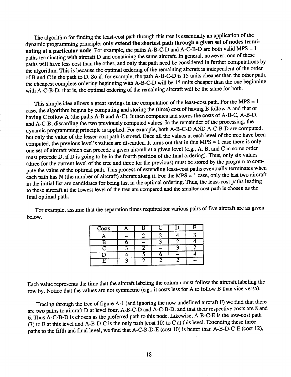
For example, assume that the separation times required for various pairs of five aircraft are as given

below.

Costs A B C D E

A - 2 2 4 3

B 6 - 3 2 4

C 3 2 - 3 2

D 4 5 6 - 4

E 3 2 2 2 -

Each value represents the time that the aircraft labeling the column must follow the aircraft labeling the

row by. Notice that the values are not symmetric (e.g., it costs less for A to follow B than vice versa).

Tracing through the tree of figure A- 1 (and ignoring the now undefined aircraft F) we find that there

are two paths to aircraft D at level four, A-B-C-D and A-C-B-D, and that their respective costs are 8 and

6. Thus A-C-B-D is chosen as the preferred path to this node. Likewise, A-B-C-E is the low-cost path

(7) to E at this level and A-B-D-C is the only path (cost 10) to C at this level. Extending these three

paths to the fifth and final level, we find that A-C-B-D-E (cost 10) is better than A-B-D-C-E (cost 12),

but A-B-C-E-D is preferable to both of these (cost 9). This f'mal path is therefore chosen as the overall

optimal path.

An additional detail of the algorithm, which has so far been neglected, is the maintenance of the list

of best paths to each node of the search tree. This can be handled in a number of ways; a particularly

simple way for the MPS = 1 case is to simply maintain three vectors that represent the best path thus far

to the leftmost, middle, and rightmost nodes of the tree. For example, when A-C-B is chosen as the best

path to D at level four in the example above, this path (the leftmost path at level three) can be copied to

the vector for the middle path (position of D at level four) and D can be appended. Of course, care must

be taken not to overwrite a vector representing a path at the previous level before that level has been

completely processed, so two sets of three vectors (one for current level and one for previous) can be

used.

APPENDIX B

COMBINED FCFS AND TIME-ADVANCE ALGORITHM

The combined FCFS and time-advance algorithm uses aircraft data as input. It is called once every

time a new aircraft enters the Center air space. Because of the different lengths of the flightpaths, the

aircraft are not in the landing order. The input data set for each aircraft consist of aircraft type (heavy or

large), ETA, and route identification. The output data consist of STA. The algorithm schedules the air-

craft and puts out arrays of aircraft data that are in the order of STAs. The aircraft with the highest index

'T' is the aircraft to land last, provided no other aircraft enter the Center. When the first aircraft enters

the Center air space, the index i = 0 is assigned and STA = ETA. The STA calculations include a time-

advance, TA = 1 minute, if selected. An aircraft can be time advanced if it follows a scheduling gap,

thus having no delay, and the following aircraft has an original SLT that is a minimum time-interval,

dtmin, ahead. The remainder of the algorithm description is without time-advance. TA is treated in the

last paragraph.

To calculate the STAs, the time-separation matrix for the succession of various aircraft classes is

needed (given in the section on Scheduling Algorithms in the main text).

As a new aircraft enters the Center air space (ith aircraft) we first check if it has an ETA greater

than that of the last (and largest) scheduled STA. In this case we assign STA[i] = ETA[i], provided

the separation is equal to or larger than the minimum separation time dtmin for the two types of

aircraft. If it is not, we delay the newcomer so that it will have the minimum allowable spacing

(STA[i] = STA[i - 1] + dtmin).

If the newly arrived aircraft has an ETA smaller than the so-far-largest STA, we first search all STA

gaps up to the one that includes the ETA of the new aircraft to see if they are large enough to accommo-

date insertion of the aircraft without having to reschedule any other aircraft. To achieve this, the time

between the earlier scheduled aircraft must be larger than the sum of the appropriate dtmins if the new

aircraft were inserted. In addition, the gap between the new aircraft and the next following STA must be

equal to or larger than the appropriate minimum separation. If more than one gap fulf'dls these condi-

tions, the new aircraft is scheduled to result in the smallest delay by being inserted into the earliest pos-

sible gap, dtmin ahead of the earlier aircraft.

Sometimes, no gap is available into which the new aircraft can be inserted without rescheduling any

other aircraft. Then the new aircraft is scheduled ahead of the first aircraft that has a non-frozen schedule

and whose STA is larger than the ETA of the new aircraft. The appropriate dtmin for the last frozen

aircraft is used for the new aircraft, provided this does not require a time-advance of the new aircraft. If

the ETA of the new aircraft is larger than the frozen aircraft's largest STA, then the new aircraft's STA

is chosen to be the larger value of ETA, or STA of the next earlier aircraft plus the required minimum

distance between that aircraft and the new aircraft. All later aircraft are then rescheduled to meet the

separation standards.

PRECEDING PAGE BLAN';_; NOT FILMED

If a time-advance is desired, it is calculated simultaneously as scheduling proceeds. Whenever

we do not schedule STA = ETA, we ask if the last aircraft before the new one had this property.

If it did, this would mean that the last aircraft was following a gap and was leading a new group of

at least two aircraft. Then TA would be used to reduce the size of the gap by 1 rain if the remaining

gap was greater than dtmin, or to dtmin, if this would take less than a l-rain time-advance. Once the

last aircraft before the new one has been rescheduled (time-advanced), the new STA is calculated,

STA[i] = STA[i - 1] + dtmin.

REFERENCES

Erzberger, Heinz; and Nedell, William: Design of Automated System for Management of Arrival

Traffic. NASA TM-102201, 1989.

MagiU, S. A. N.; and Budd, A. J.: Negative Delay in the Airport Arrival Process. Proc. UKSC Con-

ference on Computer Simulation, Bangor, Sept. 1987.

MagiU, S. A. N.; Tyler, A. C. F.; Wilkinson, E. T.; and Finch, W.: Computer-Based Tools for Assist-

ing Air Traffic Controllers with Arrivals Flow Management. Report No. 88001, Royal Signals

and Radar Establishment, Malvern, Worcestershire, 1988.

Dear, R. G.: The Dynamic Scheduling of Aircraft in the Near-Terminal Area. Report R76-9, M.I.T.

Flight Transportation Laboratory, Sept. 1976.

Voelkers, Uwe: Computer-Assisted Arrival Sequencing and Scheduling with the COMPAS-System.

AIAA/ASCE International Air Transportation Conference, Dallas, Texas, June 1986.

6. Alcabin, Monica; Erzberger, Heinz; Tobias, Leonard; and O'Brien, P. J.: Simulation of Time-Control

Procedures for Terminal Area Flow Management. 1985 American Control Conference, Boston,

Mass., June 1985.

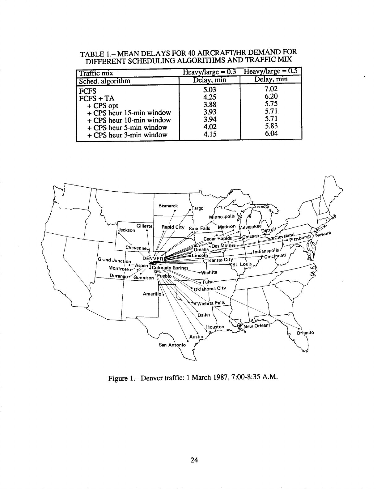
TABLE 1.- MEAN DELAYS FOR40AIRCRAFT/HR DEMAND FOR

DIFFERENTSCHEDULINGALGORITHMS AND TRAFFIC MIX

Traffic mix Heavy/larl_e = 0.3 Heavy/large = 0.5

Sched. algorithm Delay, min Delay, min

FCFS

FCFS + TA

+ CPS opt

+ CPS heur 15-rain window

+ CPS heur 10-min window

+ CPS heur 5-min window

+ CPS heur 3-rnin window

5.03

4.25

3.88

3.93

3.94

4.02

4.15

7.02

6.20

5.75

5.71

5.83

6.04

Bismarck

Gillette Rapid City

Jackson

Cheyenne

Grand Junction

MOntr, I ,_-_

DENVEF

Amarillo

Suix Falls Madison

Cedar Ra

;ansas City

ngs---_ Wichita

ils

Okll _ma City

Ir lianapO

San Antonio

Houston Jew Orleans

Orlando

Figure 1.- Denver traffic: 1 March 1987, 7:00-8:35 A.M.

t,3

C.-

0"1

i.do

t,o

= 3

• .L..,

i-=°

P_.. .=.

Number of aircraft scheduled to land

L J ! L___

i I

r-. c3

.c _

I--

-- r-

-- :3

-- O

E -

O__

E -

fj -

0}__

- E

-- ¢-

_ _

- U

._.._

°_

°_.,_

Center boundary time

I , , , , , I , , , ,

I i

90 min

I I i I i

_ Keann

_ Drako

_%_ctr boundary t

FCFS t

dly 2.12

+ TA

dly 1.21

'1 I "1'1 ' II t I"'l '"1 ''" ,

I I I

(c)

i I ' ' ' ' ' I

60 90

scheduled landing times

''II "'I'

i I i

120 min

+CPS

i ,I,,' dly1.13

I I l I

I I I I

Center boundary time

I I I I

i i I

90 min

I i

__ Keann

orate

ctr boundary t

ETA

I 'I ' ';'III I ''" '" '" ''II J'l t';"lll '" "I ""

, , t , ' ' ' ' I , , , , I ' '

60 90 120 mln

(d) scheduled landing times

FCFS t

dly 13.87

+ TA

dly 12.91

+CPS

i dly 12.91

i i I

Figure 5.- Concluded. (c) Heavy traffic, well spread out; (d) heavy traffic with large delay.

.c: _

O_ m

r,D--

E -

C O

.c: _

(,D

E -

_o_

d12

r,-

4r_

...a.

r._

°_,._

°,-4

¢.)

•

_. -- _ _

_:_:----:_- f, _

:.___ i _°

le--

(1)

-1-

__ "t"

--4 C%1

_-- + II

--4

_4 C_I

"4 II

--4- i

4 --4, T--

:_::.<_ -- + II

--;, C_l

-'_ II

_4 , "1"

":9"

i,-

"_ 0

=.o

0 G)

+ II II

c-_ C).

"E "E

o,_,1

///I

SEED was 109

i I

I t

(a)

III

1111

'1'1

III

i , i i I i I i i

I i

I I i I

(bl)

I I

+ TA

CPS 386.80

+CPS

(b)

SEED was 109

iili

I I I I

I I I

'ltll

'"'1 I =

' I

(al)

I I I I I I I I

(b2)

I I I I I t

t/ + TA

CPS 318.26

+CPS

I = I I

(c)

SEED was 109

IIII I

I , ,_ ,1,1,11 ,

I I I I I

(a2) b3)

90 120 min

scheduled landing times [heuristic CPS]

I + TA

dly 6.45

CPS 321.87

+CPS

dly 5.36

i i I

Figure 9.- Comparison of two versions of post-processing of the optimal CPS and the heuristic CPS.

(a) Optimal CPS, remove all position switches in a group if one negative delay <-1 min exists:

SEED 109; (b) optimal CPS, keep all position switches but reduce negative delay to <-1 min:

SEED 109; (c) heuristic CPS, locally proposed switches are not made if this would result in negative

delay <-1 min: SEED 109.

(d)

sLLL J11!ffll

IIII II I

"ll II I iiii

t i i

III

/If/lIt

(cl)

I I I I I

III

I/tI/IC//

III I IIII

I I

Ill(lffltf+TA

CPS 158.97

+CPS

IIII II I II I

I ' ' I t i , , , I

IIII

SEED was 111

Illlll

IIII II

] I I

(e)

ill

Ill I I

(c2)

III

[lIlll

I II I Ill

I I I

III

+ TA

CPS 167.43

+CPS

I I l i I I i t i i i I

(f)

SEED was 111

Ill I I

i II I I '"

i I I

(c3)

I i I

fll/l//f

llll llli

III I

+ TA

CPS 158.97

+CPS

II III II i dly 2.65

120 min

scheduled landing times [heuristic CPS]

Figure 9.- Concluded. (d) Optimal CPS, remove all position switches in a group if one negative delay

<-1 min exists: SEED 111; (e) optimal CPS, keep all position switches but reduce negative delay to

<-1 min: SEED 111; (f) heuristic CPS, locally proposed switches are not made if this would result in

negative delay <-1 rain: SEED 111.

,_- .5

o .4

"5 .3

<.D

7-"

.9 _: " "-'_"_ /"

.]:,o,/, /,// i" -,, , =_

•,'1 : .'. s

.8 ,9' / / / ,i

• ::? 7 !i i I' I I

:':" - f/ I i1 t

.7 :: :i I I i i / •

• :_ : : i'l i t/ t

" ." ' i!. i , r •

.. . ., . f

.. : -!" : , i l ; ,l i

: :'" :' 1" / / ,'_l

.. .;: /,1 1 iI t_l_/ _I

. ;: /) ii .f _ FCFS

"i '1" .-"qlF.L /' "'_ FCFS+TA ---

• t/ ","

/ ! _ FCFS+TA +CPS

• .-, :.. i //

: ' "i .: i' / ,, r ": t

•. : //! :. { /

...:- ! , I i/ i

{; :_" : /i i

• ":': " l ' i

: .i " _ I ." I

:'-" ";'(" :: /;i 1 7/," 1"

" !: i.:. ,, I // l

. . _;. / ¢ ." ,'"

0 1 2 3 4 5 6 7 8

" " . ....;'-_ :Z.._" .-_c;-_.

'r" _.

-d I/,/'i..

9 10 11 12 13 14 15 16 17

Average delay per aircraft [minutes]

Figure 10.- Cumulative probability distributions for traffic and aircraft type mix best for CPS

(traffic NE/NW and heavies/large = 50%/50%) for 1.5-hr traffic samples.

:, '{,,' t

_. ,i 35 40 /_/ N = 45

:'" i:t [,t

<,,,,,

FCFS

FCFS+TA

_' FCFS+TA +CPS

8 9 10 11 12 13 14 15 16 17

: /

/i i

,,: ,,

>' .6 .l .: e" _ '[ I // f

.= . ......, : /,

o ,

s': [

_. .5 ,- . :.:. : j/. f ,"

,i1

> :. I ''f 1[ .:i / //:

.4 :,: // .

-_ . .-.-

E " I " " /:t If i J

(J .3 .... .:. _ • i

: '" k':;" ,:' /' i /

" "2 ,: t

.. ,';" : _':

.2 : ,_'

• . .: ,_, /

: : "I _ ,#: t" #/_ i/

.1: ':: ' : :: // / // /

1 2 3 4 5 6 7

Average delay per aircraft [minutes]

Figure 11.- Cumulative probability distributions for nominal traffic and aircraft type mix

NE/NW traffic 66.66%/33.33%, large/heavy = 70%/30%) for 1.5-hr traffic samples.

°_

.I2

o's

•>- .4

i ,//

I/ /I-..._ _i' t

: : I :_-'7_...._."

[ i f •

ii i // i

:,: : i

: / /

: ' 1/ I

s i ' i

.:,;: /i !

.,': i I i ,.

:i : ,"i I

,"_ <

ii ;/ J

'" : i,, ,i,

,,."; .i _i"

,':,,'iI ,S.- ,,i

,:: ,,/ :

J: :!l :

,/i .< ," /

i:I:i:./

1 2 3 4 5 6 7 8 9 10

Average delay per aircraft [minutes]

"----" .5 heavy

.5 large

.3 heavy

.7 large

11 12 13

Figure 12.- Comparison of cumulative distributions for different traffic and aircraft mixes, 1.5-hr

samples, 40 aircraft/hr.

1°

=-.

_.6

°m

,.Q

.o .5

0 1

s;x, l

i)ii "

I/ _

'_1

!, !

=';,;I

k '____. FCFS

:'_ _ _ FCFS+TA

i,, _, _ FCFS+TA+CPS i

s,':' _ FCFS+TA+CPS w overtake

.:, t .,'

if;'

i .'[,' ,,,

J'," I"

-i_i i

:; ; i":

D:! i'

D" ,

2 3 4 5 6 7 8 9

Average delay per aircraft [minutes]

10 11 12

Figure 13.- Cumulative distribution for nominal traffic, 40 aircraft/hr including CPS with overtake.

(a) Optimal CPS performance.

//,

.2 ' t;'

,1 -- /

'/ /

I /

f/X

// /

/_ ,_I FCFS

- _--,_"1FCFS.TA

/ F"l FCFS+TA+CPS(heuristcs)

_ _ FCFS+TA+CPS(0ptimal)

t. " ': ; both CPS w overtake

_: ' I

" Li

¢:,/ ,

'!;

/ I

./ .61 opt CPS---i_r._',i'i_:_"

/": .5_1_5s@:i::::ii':::'8"°_:::/.[:::,' ...."'............

3_I:;FC_÷,A:,_FCFS

.4 .:;';".'"_" ,

4 5

0 1 2 3 4 5 6 7 8 9 10 11

Average delay per aircraft [minutes]

Figure 13.- Concluded. (b) Showing slight decrease in performance for the heuristics CPS vs optimal

CPS. Inset shows performance as function of scheduling window size in minutes.

1°

.i .6

..Q

9 .5

O .3

0 1 2 3 4 5 6 7

11.5.rI

8 9 10 11 12 13 14 15

Average delay per aircraft [minutes]

Figure 14.- Effect of length of the traffic sample with otherwise same statistical parameters as shown in

figure 13.

3 4 5 6 7 8

Average delay per aircraft [minutes]

Figure 15.- Effect of changing freeze horizon.

y=16

3.0 hr

1.0 hr

.5 hr

.25 hr

0 I I I I

25 30 35 40 45

Scheduled arrival rate (no. of aircraft/hr)

Figure 16.- Delay as function of traffic sample length.

y= 16

1.5 hr triangle

1.5 hr rectan

0.5 hr triangle

0.5 hr rectangle

I I I I

30 35 40 45

Scheduled arrival rate (no. of aircraft/hr)

Figure 17.- Increase of delay triangular vs rectangular distributions.

y= 16

1.5 hr samples

20 knot wind

._c

1.5 hr samples

0 knot wind

0.5 hr samples

20 knot wind

0.5 hr samples

0 knot wind

I I I I

30 35 40 45

Scheduled arrival rate (no. of aircraft/hr)

Figure 18.- Increased delays with headwind for rectangular traffic distributions.

y=14

.E 10

._ 5

distributions of preferred landing times

.3 min in trail

0 ) 90 120 min

I I I I

25 30 35 40 45

Scheduled arrival rate (no. of aircraft/hr)

Figure 19.- Effect of variable in-trail spacing.

B C

B C D

D E F

e u n

a n e

r s x

I h t

i i

e f

r t

Figure A- 1.- Illustration of all possible re-orderings of aircraft, given initial ordering A-B-C-D-E-....

N/LSA

Nslo_l Aef_au_cs amd

I.ReportNo.

NASA TM- 102795

Report Documentation Page

2. Government Accession No.

4. Title and Subtitle

Analysis of Sequencing and Scheduling Methods for Arrival

Traffic

7. Author(s)

Frank Neuman and Heinz Erzberger

9. Performing Organization Name and Address

Ames Research Center

Moffett Field, CA 94035-1000

12. Sponsoring Agency Name and Address

National Aeronautics and Space Administration

Washington, DC 20546-0001

3. Recipienrs Catalog No.

5. Report Date

April 1990

6. Performing Organization Code

8. Performing Organization Report No.

A-90086

10. Work Unit No.

505-67-21

11. Contract or Grant No.

13. Type of Report and Period Covered

Technical Memorandum

14. Sponsoring Agency Code

15. Supplementary Notes

Point of Contact: Frank Neuman, Ames Research Center, MS 210-9, Moffett Field, CA 94035-1000

(415) 604-5437 or FTS 464-5437

16. Abstract

The air traffic control subsystem that performs scheduling is discussed. The function of the schedul-

ing algorithms is to plan automatically the most efficient landing order and to assign optimally spaced

landing times to all arrivals. Several important scheduling algorithms are described and the statistical

performance of the scheduling algorithms is examined. Scheduling brings order to an arrival sequence for

aircraft. First-come-first-served scheduling (FCFS) establishes a fair order, based on estimated times of

arrival, and determines proper separations. Because of the randomness of the traffic, gaps will remain in

the scheduled sequence of aircraft. These gaps are filled, or partiaUy filled, by time-advancing the leading

aircraft after a gap while still preserving the FCFS order. Tightly scheduled groups of aircraft remain with

a mix of heavy and large aircraft. Separation requirements differ for different types of aircraft trailing each

other. Advantage is taken of this fact through mild reordering of the traffic, thus shortening the groups and

reducing average delays. Actual delays for different samples with the same statistical parameters vary

widely, especially for heavy traffic.

17. Key Words (Suggested by Author(s))

Air traffic control

Aircraft scheduling

Aircraft sequencing

19. Security Classif. (of this report)

Unclassified

18. Distribution Statement

Unclassified-Unlimited

Subject Category - 03

20. Secudty Classif. (of this page)

Unclassified

21. No. of Pages

22. Price

A03

NASA FORM 1626 OCT86

For sale by the National Technical Information Service, Springfield, Virginia 22161