The Spoken British National Corpus 2014

ROBBIE LOVE

Design, compilation and analysis

ESRC Centre for Corpus Approaches to Social Science

Department of Linguistics and English Language

Lancaster University

A thesis submitted to Lancaster University

for the degree of Doctor of Philosophy in Linguistics

September 2017

i 
 
Contents 
Contents ............................................................................................................. i 
Abstract ............................................................................................................. v 
Acknowledgements ......................................................................................... vi 
List of tables .................................................................................................. viii 
List of figures .................................................................................................... x 
Introduction ............................................................................................... 1 
1  Overview .................................................................................................................................... 1 
2  Research aims & structure ....................................................................................................... 3 
Literature review ........................................................................................ 6 
1  Introduction ............................................................................................................................... 6 
2  The Spoken British National Corpus 1994 & other spoken corpora ............................... 7 
2.1  The Spoken BNC1994 ...................................................................................................... 7 
2.2  Other British English corpora containing spoken data ................................................ 9 
2.3  Summary and justification for the Spoken BNC2014 ................................................ 11 
3  Review of research based on spoken English corpora ...................................................... 12 
3.1  Introduction ...................................................................................................................... 12 
3.2  Corpus linguistics journals .............................................................................................. 13 
3.3  Grammars ......................................................................................................................... 18 
4  Summary .................................................................................................................................. 20 
Corpus design .......................................................................................... 22 
1  Introduction ............................................................................................................................. 22 
2  Design & speaker recruitment .............................................................................................. 22 
2.1  ‘Demographic’ corpus data ............................................................................................. 22 
2.2  Design of the Spoken BNC1994DS ............................................................................. 23 
2.3  Speaker recruitment in the Spoken BNC1994 ............................................................. 27 

ii 
 
2.4  Design & recruitment in other spoken corpora .......................................................... 29 
2.5  General approach to design in the Spoken BNC2014 ............................................... 31 
2.6  Speaker recruitment in the Spoken BNC2014 ............................................................. 33 
3  Speaker and text metadata ..................................................................................................... 37 
3.1  Introduction ...................................................................................................................... 37 
3.2  Metadata in the Spoken BNC1994 ................................................................................ 38 
3.3  Metadata collection in the Spoken BNC2014: procedure and ethics ....................... 41 
3.4  Speaker & text metadata collection procedures in the Spoken BNC2014 .............. 46 
3.5  Age, linguistic region & socio-economic status: discussion ...................................... 48 
4  Collection of audio data ......................................................................................................... 70 
4.1  Introduction ...................................................................................................................... 70 
4.2  Audio recording in the Spoken BNC1994 ................................................................... 70 
4.3  Audio recording in the Spoken BNC2014 ................................................................... 70 
5  Chapter summary .................................................................................................................... 76 
Transcription ........................................................................................... 77 
1  Introduction ............................................................................................................................. 77 
2  Transcription: human vs. machine ....................................................................................... 77 
3  Approach to human transcription ........................................................................................ 83 
4  The Spoken BNC1994 transcription scheme ..................................................................... 87 
5  The Spoken BNC2014 transcription scheme: main features ........................................... 88 
6  The Spoken BNC2014 transcription process ..................................................................... 98 
7  Chapter summary .................................................................................................................. 100 
Speaker identification ............................................................................. 102 
1  Introduction ........................................................................................................................... 102 
2  Speaker identification ........................................................................................................... 102 
3  Pilot study .............................................................................................................................. 106 
3.1  Pilot study (A): Certainty (pilot study recordings) .................................................... 106 

iii 
 
3.2  Pilot study (B): Certainty (Spoken BNC2014 recording) ......................................... 107 
3.3  Pilot study (C): Inter-rater agreement (Spoken BNC2014 recording) ................... 107 
4  Research Questions .............................................................................................................. 108 
5  Methodological approach .................................................................................................... 109 
5.1  Introduction .................................................................................................................... 109 
5.2  Main study (A): a Spoken BNC2014 recording ......................................................... 110 
5.3  Main study (B): the gold standard recording.............................................................. 111 
6  Results .................................................................................................................................... 113 
6.1  Main study (A1): Certainty in a Spoken BNC2014 recording ................................. 113 
6.2  Main study (A2): Inter-rater agreement in a Spoken BNC2014 recording............ 114 
6.3  Main study (B1): Certainty in the gold standard recording ...................................... 115 
6.4  Main study (B2): Inter-rater agreement in the gold standard recording ................ 116 
6.5  Main study (B3): Accuracy in the gold standard recording ...................................... 118 
7  Discussion: what does this mean for the Spoken BNC2014? ........................................ 119 
7.1  Individual transcriber variation .................................................................................... 120 
7.2  Automated speaker identification ................................................................................ 120 
7.3  The use of phonetic expertise ...................................................................................... 122 
8  Affected texts and solutions implemented ........................................................................ 123 
9  Chapter summary .................................................................................................................. 125 
Corpus processing and dissemination ................................................... 128 
1  Introduction ........................................................................................................................... 128 
2  XML conversion ................................................................................................................... 128 
3  Annotation ............................................................................................................................. 133 
4  Corpus dissemination ........................................................................................................... 136 
5  Chapter summary .................................................................................................................. 141 
Analysing the Spoken BNC2014 ............................................................. 142 
1  Introduction ........................................................................................................................... 142 

iv 
 
2  Swearing in linguistics .......................................................................................................... 143 
2.1  Swearing as an object of study ..................................................................................... 143 
2.2  Defining swearing .......................................................................................................... 144 
2.3  McEnery’s approach to bad language ......................................................................... 146 
3  Method ................................................................................................................................... 148 
3.1  Methodological procedure ............................................................................................ 148 
3.2  Data .................................................................................................................................. 151 
4  Results .................................................................................................................................... 154 
4.1  Frequency comparison .................................................................................................. 154 
4.2  Strength ........................................................................................................................... 155 
4.3  Change and stability in frequency ................................................................................ 161 
4.4  High-frequency BLWs: sociolinguistic distribution .................................................. 165 
4.5  Sociolinguistic distribution ........................................................................................... 166 
4.6  Case study: linguistic annotation of FUCK ............................................................... 173 
5  Chapter summary .................................................................................................................. 178 
Conclusion .............................................................................................. 181 
1  Overview of the thesis ......................................................................................................... 181 
2  Successes, limitations & recommended future work ....................................................... 185 
3  Summary ................................................................................................................................ 188 
References ..................................................................................................... 189 
List of Appendices ........................................................................................ 207 
Appendices ................................................................................................... 208 
 

Abstract

The ESRC-funded Centre for Corpus Approaches to Social Science at Lancaster

University (CASS) and the English Language Teaching group at Cambridge University Press

(CUP) have compiled a new, publicly-accessible corpus of spoken British English from the

2010s, known as the Spoken British National Corpus 2014 (Spoken BNC2014). The 11.5

million-word corpus, gathered solely in informal contexts, is the first freely-accessible corpus of

its kind since the spoken component of the original British National Corpus (the Spoken

BNC1994), which, despite its age, is still used as a proxy for present-day English in research

today.

This thesis presents a detailed account of each stage of the Spoken BNC2014’s

construction, including its conception, design, transcription, processing and dissemination. It

also demonstrates the research potential of the corpus, by presenting a diachronic analysis of

‘bad language’ in spoken British English, comparing the 1990s to the 2010s. The thesis shows

how the research team struck a delicate balance between backwards compatibility with the

Spoken BNC1994 and optimal practice in the context of compiling a new corpus. Although

comparable with its predecessor, the Spoken BNC2014 is shown to represent innovation in

approaches to the compilation of spoken corpora.

This thesis makes several useful contributions to the linguistic research community. The

Spoken BNC2014 itself should be of use to many researchers, educators and students in the

corpus linguistics and English language communities and beyond. In addition, the thesis

represents an example of good practice with regards to academic collaboration with a

commercial stakeholder. Thirdly, although not a ‘user guide’, the methodological discussions and

analysis presented in this thesis are intended to help the Spoken BNC2014 to be as useful to as

many people, and for as many purposes, as possible.

Acknowledgements

This work would not have been possible without the help, support and generosity of

many people around me. First and foremost, I have been very lucky to have had as my

supervisor Tony McEnery. He pushed me to break through the many mental barriers I inflicted

upon myself, and I will take with me many of the wisdoms he has imparted on me. I must also

single out Andrew Hardie, who in many ways was my unofficial second supervisor. I am grateful

for all the support and guidance he has given me throughout my studies. Together, it was Tony

and Andrew who recruited me to work on this project, and I am extremely grateful for this and

all other opportunities they have afforded me.

I am also very grateful to the rest of the Spoken BNC2014 research team. Claire Dembry

at Cambridge University Press has been a brilliant colleague and friend, providing inspiration and

support throughout the project. Her team at CUP, including Olivia Goodman, Imogen Dickens,

Sarah Grieves and Laura Grimes, did much of the front-line work on the project and I am truly

grateful for their cooperation and expertise. Vaclav Brezina at Lancaster University has also

helped me greatly over the last four years as a collaborator on this and several other projects.

I have many reasons to thank both the ESRC-funded Centre for Corpus Approaches to

Social Science (CASS) and the Department of Linguistics and English Language (LAEL) at

Lancaster University. Many at CASS have had a hand in my professional and personal

development during the course of this work, including: Jennifer Hughes, Amelia Joulain-Jay,

Amanda Potts, Mark McGlashan, Ruth Avon, Sheryl Prentice and Paul Baker. I am grateful to

many of the academic staff at LAEL, including: Jonathan Culpeper, who as my confirmation

panellist provided very useful feedback; Sam Kirkham, who provided insights from phonetics so

readily; and the department’s administrative staff, who provided excellent support. My thanks

also extend to Matty Robinson and Gavin Brookes, who proofread much of this thesis.

As I approached the final months of writing up this thesis, I moved to Cambridge to

start working at Cambridge Assessment English. I am grateful to colleagues there who supported

me while I balanced my new role with my remaining PhD work.

One of my favourite hobbies is performing at the theatre. I am grateful to the members

of several theatre groups – Lancaster University Theatre Group, Lancaster Amateur Dramatic

and Operatic Society, About Theatre, the Morecambe Warblers and, most recent, Cambridge

Operatic Society – who welcomed me and allowed me to blow off steam in some glitzy musical.

vii

I am also indebted to friends who have shown an interest in my work, argued with me

about language, and most importantly motivated me to keep going – thank you most of all to

Matthew Bosley, Gavin Brookes, Mathew Gillings and Niall Curry.

Finally, I must thank my parents – Janet and Geoff – for providing love and support

during difficult periods of this work, and always being there to listen. I am also grateful to the

rest of my family for their enduring enthusiasm, interest and pride in my work. This thesis is

dedicated to my family, with love.

Robbie Love

Cambridge, UK

September 2017

viii 
 
List of  tables 
Table 1. Proportion of selected articles relative to the total number of articles published by each journal between 1994 and 2016. .................................. 14 
Table 2. Proportions of words in Spoken BNC1994 assigned across each of the three selection criteria (adapted from Burnard 2000: 13). .................... 25 
Table 3. Approach to corpus design taken by the compilers of a variety of spoken corpora. .................................................................................................... 30 
Table 4. Number of words categorised as ‘unknown’ or ‘info missing’ for the three main demographic categories in the Spoken BNC1994DS and the 
Spoken BNC2014. .................................................................................................................................................................................................................................. 43 
Table 5. National Readership Survey Social Grade classifications (NRS 2014). ........................................................................................................................... 63 
Table 6. Social Class based on Occupation (SC) (Stuchbury 2013b). ............................................................................................................................................. 64 
Table 7. Socio-economic group (SEG) (Stuchbury 2013a). ............................................................................................................................................................. 65 
Table 8. The nine major analytic classes of the NS-SEC (ONS 2010c). ........................................................................................................................................ 66 
Table 9. Mapping between the NS-SEC and Social Grade assumed for Spoken BNC2014 speaker metadata. ...................................................................... 69 
Table 10. List of permissible filled pauses in the Spoken BNC2014 transcription scheme. ....................................................................................................... 95 
Table 11. Speaker metadata for the gold standard recording. ........................................................................................................................................................ 112 
Table 12. Distribution of code types in the Spoken BNC2014 transcripts. ................................................................................................................................. 114 
Table 13. Total distribution of code types for the eight Spoken BNC2014 transcripts. ............................................................................................................ 115 
Table 14. Distribution of code types in the gold standard transcripts. ......................................................................................................................................... 116 
Table 15. Total distribution of code types for the eight gold standard test transcripts. ............................................................................................................. 117 
Table 16. Categories of speaker ID code for which agreement between the gold standard and test transcripts could occur. ............................................ 118 
Table 17. Inter-rater agreement (i.e. accuracy) of speaker identification between the test transcripts and the gold standard transcript. .......................... 119 
Table 18. Accuracy of the phonetician’s transcript compared to the gold standard test transcript extracts. .......................................................................... 123 
Table 19. Frequency of corpus texts per number of speakers per recording in the Spoken BNC2014. ................................................................................. 124 

ix 
 
Table 20. LCA annotation scheme (McEnery 2005: 27); modifications are italicised. ............................................................................................................... 147 
Table 21. Categories of insult in the LCA annotation scheme (McEnery 2005: 27). ................................................................................................................. 147 
Table 22. Token counts for the groups within demographic categories gender, age and socio-economic status in the Spoken BNC1994DS and Spoken 
BNC2014S. ............................................................................................................................................................................................................................................ 152 
Table 23. A scale of offence (McEnery 2005: 30). ........................................................................................................................................................................... 156 
Table 24. Scale of offence for bad language (Ofcom 2016: 3). ...................................................................................................................................................... 157 
Table 25. BLWs in the Ofcom (2016) report, which are given unambiguous ratings in the scale of offence. ....................................................................... 157 
Table 26. BLWs which have decreased in use significantly (p<0.0001) between the 1990s and 2010s, ranked by effect size. ........................................... 163 
Table 27. BLWs which have increased in use significantly (p<0.0001) between the 1990s and 2010s, ranked by effect size. ............................................ 164 
Table 28. BLWs which have not changed in frequency significantly (p>0.05) between the 1990s and 2010s, and which have a minimum raw frequency 
of 100 in both corpora, ranked alphabetically. ................................................................................................................................................................................. 165 
Table 29. Annotation of FUCK in the Spoken BNC1994DS and the Spoken BNC2014S, using the bad language categorization scheme. ................... 175 
Table 30. Information about the recordings used in the speaker identification investigations. ................................................................................................ 258 
 
 

x 
 
List of  figures 
Figure 1. Comparison of gender distribution between the Spoken BNC1994 speakers (Burnard 2000: 13) and the UK (England, Wales and Scotland) 
population of “present residents: in households” in 1991 (NOMIS wizard query)...................................................................................................................... 26 
Figure 2. Comparison of age distribution between the Spoken BNC1994DS speakers (Burnard 2000: 13) and the UK (England and Wales only) 
population in 1991 (NOMIS wizard query). ....................................................................................................................................................................................... 27 
Figure 3. The Spoken BNC1994DS’s geographic regions (reproduced from Crowdy 1993: 260). ............................................................................................ 28 
Figure 4. Example of an online news article reporting on early findings from the Spoken BNC2014. .................................................................................... 34 
Figure 5. The relationship between researcher, contributor and speaker when compiling a spoken corpus (double-headed arrows indicate contact 
between the linked parties; dotted lines indicate that n is a theoretically unknown number that is only known in practice). ............................................... 36 
Figure 6. Example of conversation log given to contributors in the Spoken BNC1994DS (reproduced from Crowdy 1993: 260). ................................... 40 
Figure 7. The Speaker Information Sheet/consent form used in the Spoken BNC2014. ........................................................................................................... 42 
Figure 8. Recording Information Sheet used in the Spoken BNC2014. ........................................................................................................................................ 45 
Figure 9. Dialect categories used in the Spoken BNC1994DS. ....................................................................................................................................................... 56 
Figure 10. Birthplace and dialect categories used in the Spoken BNC2014. ................................................................................................................................. 61 
Figure 11. Guidelines for Data Collection document which was provided to Spoken BNC2014 contributors. ..................................................................... 75 
Figure 12. Concordance plot of ‘[quot=’ tags in the pilot corpus (displayed in AntConc, Anthony 2014). ............................................................................. 98 
Figure 13. Proportion of indeterminable speaker identification in the pilot study corpus according to the number of speakers per recording. ............. 107 
Figure 14. Transcript excerpt, pre- and post-XML conversion. .................................................................................................................................................... 130 
Figure 15. Vocalisation checking functions in the XML conversion PHP script. ...................................................................................................................... 131 
Figure 16. Standard query menu for the Spoken BNC2014 in CQPweb (Hardie 2012). .......................................................................................................... 137 
Figure 17. Concordance lines for the simple query ‘love’ in the Spoken BNC2014. ................................................................................................................. 138 

xi 
 
Figure 18. Relative frequency comparison of BLWs categorised according to the Ofcom (2016) scale of offence. ............................................................ 158 
Figure 19. Gender and socio-economic status. ................................................................................................................................................................................ 160 
Figure 20. Gender and age. .................................................................................................................................................................................................................. 161 
Figure 21. Age and socio-economic status. ....................................................................................................................................................................................... 161 
Figure 22. Distribution of relative frequencies for the 12 BLWs by gender in the Spoken BNC1994DS and Spoken BNC2014S. .................................. 167 
Figure 23. Distribution of relative frequencies for the 12 BLWs by age in the Spoken BNC1994DS and Spoken BNC2014S. ........................................ 169 
Figure 24. Distribution of relative frequencies for the 12 BLWs by socio-economic status in the Spoken BNC1994DS and Spoken BNC2014S. ....... 171 
Figure 25. Distribution of the 12 BLWs in the Spoken BNC2014S according to NS-SEC. ..................................................................................................... 172 
Figure 26. Separating the turns from their corresponding speaker ID codes (invented data). ................................................................................................. 251 
Figure 27. Viewing each transcript of the same recording alongside each other (invented data). ............................................................................................ 251 
Figure 28. The speaker ID codes from each transcript after their corresponding turns have been removed (invented data). ............................................ 252 
Figure 29. Unaligned extract from original transcript and test transcript #1. ............................................................................................................................. 253 
Figure 30. Aligned extract from original transcript and test transcript #1. ................................................................................................................................. 253 
Figure 31. Unaligned extract from original transcript and test transcript #8. ............................................................................................................................. 254 
Figure 32. Aligned extract from original transcript and test transcript #8. ................................................................................................................................. 254 
Figure 33. Unaligned extract from original transcript and test transcript #1. ............................................................................................................................. 254 
Figure 34. Aligned extract from original transcript and test transcript #1. ................................................................................................................................. 255 
Figure 35. Aligned extract from original transcript and test transcript #6. ................................................................................................................................. 256 
Figure 36. Unaligned extract from original transcript and test transcript #6. ............................................................................................................................. 256 
Figure 37. Aligned extract from original transcript and test transcript #6. ................................................................................................................................. 257 
 

1 Introduction

1.1 Overview

The ESRC-funded Centre for Corpus Approaches to Social Science (CASS)

at Lancaster

University and the English Language Teaching group at Cambridge University Press (CUP) have

compiled a new, publicly-accessible corpus of present-day spoken British English, gathered in

informal contexts, known as the Spoken British National Corpus 2014 (Spoken BNC2014). This

is the first publicly-accessible corpus of its kind since the spoken component of the original

British National Corpus, which was completed in 1994, and which, despite its age, is still used as

a proxy for present-day English in research today (e.g. Hadikin 2014; Rühlemann & Gries 2015).

The new corpus contains data gathered in the years 2012 to 2016. As of September 2017 it is

available publicly via Lancaster University’s CQPweb server (Hardie 2012), with the underlying

XML files downloadable from late 2018. It will subsequently form the spoken component of the

larger British National Corpus 2014, the written component of which is also under development.

The Spoken BNC2014 contains 11,422,617 million words of transcribed content, featuring 668

speakers in 1,251 recordings.

The BNC2014’s predecessor, the British National Corpus (henceforth BNC1994), is one

of the most widely known and used corpora. No orthographically transcribed spoken corpus

compiled since the release of 10-million-word spoken component of the BNC (henceforth

Spoken BNC1994) has matched it in either its size or availability. Unsurprisingly, the corpus

linguistics community has, for some time, used the Spoken BNC1994 as a proxy for ‘present-

day’ spoken British English. That this ‘go-to’ dataset is over twenty years old at the time of

writing is a problem for current and future research that needed to be addressed with increasing

urgency.

The collaboration between CASS and CUP to build the Spoken BNC2014 came about

after some years of both centres working individually on the idea of addressing this situation by

compiling a new corpus of spoken British English which could, in some way, match up to the

Spoken BNC1994.

Claire Dembry at CUP had collected two million words of new spoken data

The research presented in this thesis was supported by the ESRC Centre for Corpus Approaches to Social Science,

ESRC grant reference ES/K002155/1.

for the Cambridge English Corpus

in 2012, trialling the public participation method which was

used, along with the data itself, in the Spoken BNC2014 (see Section 3.2.5, p. 31). Meanwhile,

Tony McEnery and Andrew Hardie at Lancaster had been planning to compile a new version of

the British National Corpus and, by 2013, had recruited (a) me, to start investigating

methodological issues in compiling spoken corpora, and (b) Vaclav Brezina, to bring insights to

the project based on his use of the Spoken BNC1994 to explore sociolinguistic research

questions. Early in 2014, both CASS and CUP agreed, upon learning of each other’s work, to

pool resources and work together to build the ‘Lancaster/Cambridge Corpus of Speech’ (LCCS)

which, within a few months and with the blessing of Martin Wynne at the University of Oxford,

was renamed the Spoken British National Corpus 2014 (Spoken BNC2014). The Spoken

BNC2014 will become the spoken subcorpus of the planned British National Corpus 2014 – the

written component is being compiled by Abi Hawtin with the support of CASS and CUP, and is

due for release in 2018.

The aim of this thesis is to present an account of the design, compilation and analysis of

the Spoken BNC2014, making clear the most important decisions the research team made as we

collected, transcribed and processed the data, as well as to demonstrate the research potential of

the corpus. The underlying theme of this thesis is the maximisation of the efficiency of spoken

corpus creation in view of practical constraints, with a focus on principles of design as well as

data and metadata collection, transcription and processing. As is not unusual in corpus

construction, compromises had to be made throughout the compilation of this corpus; these are

laid out transparently. Furthermore, this thesis describes the innovative aspects of the Spoken

BNC2014 project – notably including the use of PPSR (public participation in scientific research,

Shirk et al. 2012), the introduction of new speaker metadata categorisation schemes, and

consideration of the difficulty of speaker identification at the transcription stage – among others.

While the thesis does not function as a Spoken BNC2014 ‘user guide’,

it is a thorough account

of the careful decisions that were made at each stage of development, and should be read by

users of the corpus.

The compilation of the Spoken BNC2014 was, as stated, a collaborative research project

undertaken by CASS and CUP. It was a group effort, and, in addition to my own work, this

thesis accounts for decisions made and work completed in collaboration with a team of

researchers of which I was a member. Other members of the main research team – those who,

http://www.cambridge.org/us/cambridgeenglish/better-learning/deeper-insights/linguistics-

pedagogy/cambridge-english-corpus (last accessed September 2017).

See Love et al. (2017b) for the BNC2014 user manual and reference guide.

Several of the major themes of the thesis are captured in the Spoken BNC2014 citation paper (Love et al. 2017a),

which serves as a summary of the project.

aside from myself, made decisions which shaped the course of the compilation process – were

Vaclav Brezina, Andrew Hardie and Tony McEnery (from Lancaster), and Claire Dembry and

Laura Grimes (from Cambridge). In this thesis, I use singular and plural pronouns systematically:

first person singular pronouns are used when discussing work which was conducted solely by

me, while first person plural pronouns and third person reference to “the Spoken BNC2014

research team” are used when reporting on decisions I made with the research team.

1.2 Research aims & structure

The aims of the Spoken BNC2014 project are:

(1) to compile a corpus of informal British English conversation from the 2010s which is

comparable to the Spoken BNC1994’s demographic component;

(2) to compile the corpus in a manner which reflects, as much as possible, the state of the art

with regards to methodological approach; and, in achieving steps (2) and (3);

(3) to provide a fresh data source for a new series of wide-ranging studies in linguistics and

the social sciences.

The structure of this thesis is perhaps different to most, as its focus is expressly methodological

– it comprises a series of methodological explorations, followed by one chapter which contains

linguistic analysis. Because of this, the standard approach to a thesis, where one reviews all

relevant literature at the beginning and subsequently outlines a methodological approach that

accounts for the entire project, does not fit my purpose. Accordingly, I decided to adopt a

thematic approach, addressing each stage of the compilation of the corpus in the chronological

order in which they occurred. Following a general and over-arching Literature Review (Chapter

2), which reviews the use of the Spoken BNC1994 and other relevant corpora for linguistic

research, the thesis is divided into the following chapters:

• Chapter 3: Corpus design

This chapter covers general principles of spoken corpus design including recruitment, metadata

and audio data. A major theme of this chapter is the extent to which the Spoken BNC1994 and

other relevant corpora have been compiled using a principled as opposed to opportunistic

approach, and our decision to embrace opportunism (supplemented by targeted interventions) in

the compilation of the Spoken BNC2014.

4 
 
•  Chapter 4: Transcription 
This  chapter  discusses  the  development  of  a  bespoke  transcription  scheme  for  the  Spoken 
BNC2014. It justifies the rejection of automated transcription before describing how the Spoken 
BNC2014  transcription  scheme  elaborates  and  improves  upon  that  of  its  predecessor. It also 
demonstrates the  interactivity  between  stages of  corpus compilation; the  transcription scheme 
was designed to be mapped automatically and unambiguously into XML at a later stage in the 
construction of the corpus. 
 
•  Chapter 5: Speaker identification 
This chapter reflects upon the transcription stage of the project, investigating the accuracy with 
which  transcribers  were  able  to  assign  speaker  ID  codes  to  the  utterances  transcribed  in  the 
Spoken BNC2014 – i.e. ‘speaker identification’. Its aim is to draw attention to the difficulty of 
this task for recordings which contain several speakers, and to propose ways in which users can 
avoid having potentially inaccurately assigned speaker ID codes affect their research. 
 
•  Chapter 6: Corpus processing and dissemination 
This chapter discusses the final stages of the compilation of the Spoken BNC2014, describing 
the conversion of transcripts into XML; the annotation of the corpus texts for part-of-speech, 
lemma and semantic category; and the public dissemination of the corpus. 
 
•  Chapter 7: Analysing the Spoken BNC2014 
This chapter aims to demonstrate the research potential of the Spoken BNC2014 by comparing 
(a sample of) it to the Spoken BNC1994 in a study of bad language. This study aims to reveal 
indications  that  the  frequency,  strength  and  social  distribution  of  bad  language  may  have 
changed or remained stable between the 1990s and 2010s in spoken British English. Adopting 
the approach to bad language proposed by McEnery (2005), I analyse a large set of bad language 
words (BLWs) and demonstrate the comparability of the Spoken BNC2014 with its predecessor. 
 
Finally, Chapter 8 (the conclusion) summarises the thesis and discusses the major successes and 
limitations of my work on the project, before suggesting future work which could extend the 
research capability of the corpus. 
  Before discussing how the Spoken BNC2014 was built, I will contextualise the use and 
popularity of the  original British National Corpus, and  argue how no corpus since its spoken 

component has matched the Spoken BNC1994 in terms of several key strengths which appear to

have made it as widely used as it has been. This is the aim of the next chapter.

2 Literature review

2.1 Introduction

This Literature Review aims to contextualise the situation which has arisen whereby the

collection of a second Spoken British National Corpus is necessary. It introduces the Spoken

British National Corpus 1994 and discusses its uses in the field of linguistics. It also presents the

case for compiling a second edition now. What it does not do is discuss existing corpora in terms

of design, data collection, transcription or any other feature of corpus construction which has

informed the methods for the compilation of the Spoken BNC2014 – relevant literature on these

topics will be introduced, where appropriate, in each of the methodological chapters which

follow the Literature Review.

Corpus linguistics is “a relatively new approach in linguistics that has to do with the

empirical study of ‘real life’ language use with the help of computers and electronic corpora”

(Lüdeling & Kytö 2008: v). A well-known problem afflicting corpus linguistics as a field is its

tendency to prioritise written forms of language over spoken forms, in consequence of the

drastically greater difficulty, high cost and slower speed of collecting spoken text:

A rough guess suggests that the cost of collecting and transcribing in electronic form one

million words of naturally occurring speech is at least 10 times higher than the cost of

adding another million words of newspaper text. (Burnard 2002: 6)

Contemporary online access to newspaper material means that this disparity is likely to be even

greater today than in 2002. The resulting bias in corpus linguistics towards a “very much written-

biased view” (Lüdeling & Kytö 2008: vi) of language is problematic if one takes the view that

speech is the primary medium of communication (Čermák 2009: 113), containing linguistic

variables that are important for the accurate description of language, and yet inaccessible through

the analysis of corpora composed solely of written texts (Adolphs & Carter 2013: 1). Projects

devoted to the compilation of spoken corpora are thus relatively few and far between (Adolphs

& Carter 2013: 1).

In the next section I introduce one of the few widely accessible spoken corpora of British

English, the spoken section of the British National Corpus (henceforth the Spoken BNC1994).

This is, to this day, heavily relied upon in spoken English corpus research. I show that this is due

to the scarcity and lack of accessibility of spoken English corpora that have been developed

since; the Spoken BNC1994 is still relied upon today as the best available corpus of its kind,

despite its age. This, as I will show in Section 2.2, is a problem for current and future research,

and, along with the other problems outlined, it is presented as the main justification for

producing a new spoken corpus – the Spoken BNC2014. I then consider the types of research

for which the Spoken BNC2014 will likely be used by summarising the most prominent areas of

spoken corpus research that have arisen over the last two decades (Section 2.3). I also show that

there are limitations in such previous research that provide evidence of the problems outlined

above, and that the publicly-accessible Spoken BNC2014 aims to considerably improve the

ability of researchers to study spoken British English. I conclude by outlining the main research

aims of the thesis (Section 2.4).

2.2 The Spoken British National Corpus 1994 & other spoken corpora

2.2.1 The Spoken BNC1994

The compilation of the Spoken BNC2014 is informed largely by the BNC1994’s spoken

component (see Crowdy 1993, 1994, 1995), which is “one of the biggest available corpora of

spoken British English” (Nesselhauf & Römer 2007: 297). The goal of the BNC1994’s creators

was “to make it possible to say something about language in general” (Nesselhauf & Römer

2007: 5). Thus its spoken component was designed to function as a representative sample of

spoken British English (Burnard 2007). It was created between 1991 and 1994, and was designed

in two parts: the demographically-sampled part (c. 40%) and the context-governed part (c. 60%)

(Aston & Burnard 1998).

The demographically-sampled part

– henceforth the Spoken BNC1994DS – contains

informal, “everyday spontaneous interactions” (Leech et al. 2001: 2). Its contributors (the

volunteers who made the recordings of their interactions with other speakers) were “selected by

age group, sex, social class and geographic region” (Aston & Burnard 1998: 31). 124 adult

contributors made recordings using portable tape recorders (Aston & Burnard 1998: 32), and in

most cases only the contributor was aware of the recording taking place. Contributors wore the

recorders at all times and were instructed to record all of their interactions within a period of

between two and seven days. The Spoken BNC1994DS also incorporates the Bergen Corpus of

London Teenage Language (COLT), a half-million-word sample of spontaneous conversations

among teenagers between the ages of 13-17, collected in a variety of boroughs and school

Also known as the ‘conversational part’ (Leech et al. 2001: 2).

districts in London in 1993 (Stenström et al. 2002). In the XML edition of the BNC1994 hosted

by Lancaster University’s CQPweb server (Hardie 2012), the Spoken BNC1994DS contains five

million words of transcribed conversation produced by 1,408 speakers and distributed across 153

texts.

The context-governed part

– henceforth the Spoken BNC1994CG – contains formal

encounters from institutional settings, which were “categorised by topic and type of interaction”

(Aston & Burnard 1998: 31). Unlike the Spoken BNC1994DS, the Spoken BNC1994CG’s text

types were “selected according to a priori linguistically motivated categories” (Burnard 2000: 14):

namely educational and informative, business, public or institutional and leisure (Burnard 2000: 15).

Because of the variety of text types and settings involved, the data collection procedure varied;

some conversations were recorded using the same procedure as the DS, while recordings of

some conversations (e.g. broadcast media) already existed. The Spoken BNC1994CG contains

seven million words produced by 3,986 speakers and distributed across 755 texts.

Despite certain weaknesses in design and metadata, which I discuss in Section 3.2.2 (p.

23), the Spoken BNC1994 has proven a highly productive resource for linguistic research over

the last two decades. It has been influential in the areas of grammar (e.g. Rühlemann 2006,

Gabrielatos 2011, Smith 2014), sociolinguistics (e.g. McEnery 2006, Saily 2006, Xiao & Tao

2007), conversation analysis (e.g. Rühlemann & Gries 2015), pragmatics (e.g. Wang 2005,

Cappelle et al. 2015, Hatice 2015), and language teaching (e.g. Alderson 2007, Flowerdew 2009),

among others, which are discussed in further detail in Section 2.3.2. Part of the reason for the

widespread use of the BNC1994 is that it is an open-access corpus; researchers from around the

world can access the corpus at zero cost, either by downloading the full text from the Oxford

Text Archive,

or using the online interfaces provided by various institutions including Brigham

Young University (BNC-BYU,

Davies 2004) and Lancaster University (BNCweb,

Hoffmann et

al. 2008). Yet it is undoubtedly the unique access that the Spoken BNC1994 has provided to

large-scale orthographic transcriptions of spontaneous speech that has been the key to its

success. Such resources are needed by linguists, but are expensive and time consuming to

produce and hence are rarely accessible as openly and easily as is the BNC1994.

Also known as the ‘task-oriented part’ (Leech et al. 2001: 2).

Accessible at: http://ota.ox.ac.uk/desc/2554 (last accessed September 2017).

Accessible at: http://corpus.byu.edu/bnc/ (last accessed September 2017).

Accessible at: http://bncweb.lancs.ac.uk/bncwebSignup (last accessed September 2017).

2.2.2 Other British English corpora containing spoken data

Other corpora of spoken British English exist which are similarly conversational and

non-specialized in terms of context. Although they have the potential to be just as influential as

the Spoken BNC1994DS, they are much harder to access for several reasons. Some have simply

not been made available to the public for commercial reasons. The Cambridge and Nottingham

Corpus of Discourse in English (CANCODE), for example, forms part of the Cambridge

English Corpus, which is a commercial resource belonging to Cambridge University Press and is

not accessible to the wider research community (Carter 1998: 55). Other corpora are available

only after payment of a license fee, which makes them generally less accessible. For instance,

Collins publishers’ WordBanks Online (Collins 2017) offers paid access to a 57-million-word

subcorpus of the Bank of English

(containing data from British English and American English

sources, 61 million words of which is spoken); the charges range, at the time of writing, from a

minimum of £695 up to £3,000 per year of access. Likewise, the British component of the

International Corpus of English (ICE-GB), containing one million words of written and spoken

data from the 1990s (Nelson et al. 2002: 3), costs over £400 for a single, non-student license.

Some other corpora are generally available, but sample a more narrowly defined regional

variety of English than ‘British English’. For instance, the Scottish Corpus of Texts and Speech

(SCOTS) (Douglas 2003), while free to use, contains only Scottish English and no other regional

varieties of English from the British Isles. Its spoken section, mostly collected after the year

2000, is over one million words in length and contains a mixture of what could be considered

both conversational and task-oriented data. It serves as an example of a corpus project that aimed to

produce “a publicly available resource, mounted on and searchable via the Internet” (Douglas

2003: 24); the SCOTS website

allows users immediate and free access to the corpus. It appears

to be the first project since the Spoken BNC1994 to encourage use of the data not only by

linguists but by researchers from other disciplines too:

It is envisaged that SCOTS will be a useful resource, not only for language researchers,

but also for those working in education, government, the creative arts, media, and

tourism, who have a more general interest in Scottish culture and identity. (Douglas

2003: 24)

https://www.collinsdictionary.com/wordbanks (last accessed September 2017).

http://www.ucl.ac.uk/english-usage/projects/ice-gb/iceorder2.htm (last accessed September 2017).

http://www.scottishcorpus.ac.uk/ (last accessed September 2017).

This suggests that some work has taken place since the compilation of the BNC1994 that has, at

least in part, been able to bridge the gap of open-access, spoken, British English corpus data

between the early 1990s and the present-day.

More recently, the British Broadcasting Corporation (BBC) undertook a language

compilation project that rivalled the Spoken BNC1994 both in size and range of speakers – the

BBC Voices project (Robinson 2012). BBC Voices is “the most significant popular survey of

regional English ever undertaken around the UK” (BBC Voices 2007), and was recorded in 2004

and 2005 by fifty BBC radio journalists in locations all over the UK. All together over 1,200

speakers produced a total of 283 recordings. The only public access to the data (hosted by the

British Library’s National Sound Archive)

is to the recordings themselves. Users can freely

listen to the BBC Voices recordings online, but no transcripts exist. Since this project seems

similar to the Spoken BNC1994, it could be said that the most convenient way of producing a

successor would simply be to transcribe the BBC Voices recordings and release them as a

corpus. However, there are several differences between the Spoken BNC1994 and the BBC

Voices project which make this solution inadequate. Firstly, the BBC Voices project is a dialect

survey and not a corpus project (Robinson 2012: 23); the aim of its compilers was to search for

varieties of British English that were influenced by the widest range of geographic backgrounds

as possible, including other countries (BBC Voices 2007). Furthermore, the aim of BBC Voices

was not only to record samples of the many regional dialects of spoken English, but also to

capture discourses about language itself. The radio journalists achieved this by gathering the

recordings via informal interviews with groups of friends or colleagues, and asking specific

questions (BBC Voices 2007). This, then, is not naturally occurring language in the same sense as

the Spoken BNC1994DS, and so these conversations are not comparable. Finally, even if a

corpus of BBC Voices transcripts did exist, it would already be a decade old.

In this section I have introduced several spoken corpora of British English which have

been compiled since the release of the Spoken BNC1994, and discussed restrictions with regards

to the accessibility, appropriateness or availability of the data. These restrictions appear to have

translated into a much lower level of research output using these datasets. As a crude proxy for

the academic impact of these corpora, I searched in Lancaster University’s online library system

for publications which mention them. At the time of writing, a search for CANCODE retrieves

54 publications; WordBanks Online only 45; ICE-GB 300; SCOTS 34; and BBC Voices 101. By

contrast searching for the BNC1994 identifies 3,000 publications. While an admittedly rough rule

of thumb, this quick search shows that even though conversational, non-specialized spoken

http://sounds.bl.uk/Accents-and-dialects/BBC-Voices (last accessed September 2017).

corpora that may be just as useful as the Spoken BNC1994DS have been compiled since 1994,

their limited availability, and/or the expense of accessing them, has meant that the Spoken

BNC1994 remains the most widely used spoken corpus of British English to date.

2.2.3 Summary and justification for the Spoken BNC2014

It is clearly problematic that research into spoken British English is still using a corpus

from the early 1990s to explore ‘present-day’ English. The reason why no spoken corpus since

the Spoken BNC1994 has equalled its utility for research seems to be that no other corpus has

matched all four of its key strengths:

i. orthographically transcribed data

ii. large size

iii. general coverage of spoken British English

iv. (low or no cost) public access

Each of the other projects mentioned above fails to fulfil one or more of these criteria. For

example, CANCODE is large and general in coverage of varieties of spoken British English, but

has no public access; while the SCOTS corpus is publicly-accessible, but contains only Scottish

English. The BBC Voices project, while general in coverage, is not transcribed. The Spoken

BNC2014 is the first corpus since the original that matches all four of the key criteria.

The point has been made that the age of the Spoken BNC1994 is a problem. The

problem of the Spoken BNC1994’s continued use would be lessened if it were not still treated as

a proxy for present-day English – i.e. if its use were mainly historical – but this is not the case.

For researchers interested in spoken British English who do not have access to privately held

spoken corpora this is unavoidable; the Spoken BNC1994 is still clearly the best publicly-

accessible resource for spoken British English for the reasons outlined. Yet, as time has passed,

the corpus has been used for purposes for which it is becoming increasingly less suitable. For

example, a recent study by Hadikin (2014), which investigates the behaviour of articles in spoken

Korean English, uses the Spoken BNC1994 as a reference corpus of present-day English.

Appropriately, Hadikin (2014: 7) gives the following warning:

With notably older recordings [than the Korean corpora he compiled] […] one has to be

cautious about any language structures that may have changed, or may be changing, in

the period since then.

In this respect, Hadikin’s (2014) work typifies a range of recent research which, in the absence of

a suitable alternative, uses the Spoken BNC1994 as a sample of present-day English. The dated

nature of the Spoken BNC1994 is demonstrated by the presence in the corpus of references to

public figures, technology, and television shows that were contemporary in the early 1990s:

(1) Oh alright then, so if John Major gets elected then I’ll still [unclear]

(BNC1994 KCF)

(2) Why not just put a video on?

(BNC1994 KBC)

(3) Did you see The Generation Game?

(BNC1994 KCT)

It is clear, then, that there is a need for a new corpus of conversational British English to allow

researchers to continue the kinds of research that the Spoken BNC1994 has fostered over the

past two decades. This new corpus will also make it possible to turn the ageing of the Spoken

BNC1994 into an advantage – if it can be compared to a comparable contemporary corpus, it

can become a useful resource for exploring recent change in spoken English. The Spoken

BNC2014 project enables scholars to realise these research opportunities as well as, importantly,

allowing gratis public access to the resulting corpus.

2.3 Review of research based on spoken English corpora

2.3.1 Introduction

In this section I discuss the types of linguistic research that will likely benefit from the

compilation of the Spoken BNC2014 by reviewing the most common trends in relevant

published research between 1994 – when the Spoken BNC1994 was first released – and 2016. In

section 2.3.2, I review research published in five of the most prominent journals in the field of

corpus linguistics – research that mainly required open-access spoken corpora, or at least spoken

corpora with affordable licences, in order to be completed. In section 2.3.3, I assess the role of

spoken corpora in the development of English grammars, a process in which the question of

availability to the public is irrelevant in some cases as the publisher allows the authors access to

spoken resources they possess. I conclude that there are limitations in the research, caused by the

John Major was Prime Minister of the United Kingdom between 1990 and 1997.

The VHS tape cassette, or ‘video’, was a popular medium for home video consumption in the 1980s and 1990s

before the introduction of the DVD in the late 1990s.

The Generation Game was a popular British television gameshow which was broadcast between 1971 and 2002.

problems outlined in the previous section, which could be addressed by the compilation of the

Spoken BNC2014.

2.3.2 Corpus linguistics journals

The aim of this section is to critically discuss a wide-ranging selection of published

research based on spoken corpora (of conversational British English and other language

varieties). The purpose of this is to discuss the extent to which:

(a) spoken corpora have been found to be crucial to the advancement of knowledge in a

range of areas of research;

(b) there are avenues of research that could be ‘updated’ by new spoken data; and,

therefore,

In the case of the Spoken BNC1994, Leech (1993: 10) predicted that the corpus would be

particularly useful for “linguistic research, reference publishing, natural language processing by

computer, and language education”. This section aims to assess how this corpus, and other

corpora containing spoken data, has actually been put to use in published research. To do this I

searched the archives of five of the most popular journals which publish research in corpus

linguistics

(the dates in parentheses refer to the year in which the journals were established):

• International Computer Archive of Modern and Medieval English (ICAME) Journal (1979-)

• Digital Scholarship in the Humanities (DSH) Journal (formerly Literary and Linguistic

Computing) (1986-)

• International Journal of Corpus Linguistics (IJCL) (1996-)

• Corpus Linguistics and Linguistic Theory (CLLT) Journal (2005-)

• Corpora Journal (2006-)

For the ICAME and DSH journals, I considered only the volumes that were published from the

year 1994 and onwards; for the other three journals I searched all volumes. I chose 1994 as the

starting point because it is year that the BNC1994 was completed and began to be made publicly

By selecting only the output of five journals from the years 1994-2016, I am ignoring the many other outlets,

including monographs, edited collections and conference proceedings, that contain original spoken corpus research.

The purpose of this choice is simply to illustrate the ways in which existing spoken corpora have been used, and to

attempt to predict the types of research for which the Spoken BNC2014 may be used.

available for research (Burnard 2002: 10). Since the Spoken BNC1994 was “the first corpus of its

size to be made widely available” (Burnard 2002: 4), corpus research into spoken language prior

to the BNC1994’s publication used smaller bodies of data that were harder to access from

outside their host institution. Such research, therefore, is harder to verify and compare to more

recent spoken corpus studies, and so 1994 was the most appropriate place to start my search.

I retrieved papers that draw upon spoken corpora containing conversational data,

omitting those that drew upon data which would be considered exclusively task-oriented (in

Section 3.1, p. 22, I explain the rationale behind our choice to gather only conversational data for

the Spoken BNC2014). However, articles that draw upon corpora containing both types (e.g. the

Spoken BNC1994) were included. Likewise, I included research that used a mixture of spoken

and written corpora; the findings from the spoken data were considered relevant to my aim (I

found that many articles use corpora of written and spoken data together as a whole). The

following review is based upon the research of a total of 140 papers, published by the five

journals between the years 1994-2016. As shown in Table 1, this represents 14.23% of all articles

(excluding editorials and book reviews) published by these journals in this period, and the

highest relative frequency of articles selected for this review was generated by Corpus Linguistics

and Linguistic Theory (20.93%).

Table 1. Proportion of selected articles relative to the total number of articles published by each

journal between 1994 and 2016.

Journal

Freq. selected

articles

Freq. articles

(1994-2016)

% of all articles

(1994-2016)

ICAME

125

18.40

DSH

707

0.99

IJCL

372

18.55

CLLT

129

20.93

Corpora

114

12.28

Total

140

1447

14.23

Firstly, it is evident that spoken data has been relied upon in a considerable proportion of

(corpus) linguistic research; based on the research articles retrieved in my search, much appears

to have been said about the nature of spoken language. Secondly, it appears that research is

dominated by the English language; 117 out of the 140 studies use at least one corpus containing

some variety of English. Of these, 77% use British English data. It is not clear whether this

reflects in part the early domination of British English in the field of English Corpus Linguistics

(ECL) (McEnery & Hardie 2012: 72), or whether these journals happen to favour publishing

research which includes British English data, or both. Despite this, there has been considerable

research on spoken corpora of other languages, including:

• Belgian Dutch (Grondelaers & Speelman 2007)

• Brazilian Portuguese (Berber Sardinha et al. 2014)

• Columbian Spanish (Brown et al. 2014)

• Danish (Henrichsen & Allwood 2005, Gregersen & Barner-Rasmussen 2011)

• Dutch (Mortier & Degand 2009, Defranq & de Sutter 2010, van Bergen & de Swart

2010, Tummers et al. 2014, Rys & de Cuypere 2014, Hanique et al. 2015)

• Finnish (Karlsson 2010, Helasvuo & Kyröläinen 2016)

• French (Mortier & Degand 2009, Defranq & de Sutter 2010)

• German (Karlsson 2010, Schmidt 2016)

• Korean (Kang 2001, Oh 2005, Kim 2009, Hadikin 2014)

• Mandarin Chinese (Tseng 2005, Xiao & McEnery 2006, Wong 2006)

• Māori (King et al. 2011)

• Nepali (Hardie 2008)

• Norwegian (Drange et al. 2014)

• Russian (Janda et al. 2010)

• Slovene (Verdonik 2015)

• Spanish (Sanchez & Cantos-Gomez 1997, Butler 1998, Trillo & García 2001, de la Cruz

2003, Biber et al. 2006, Santamaría-García 2011, Drange et al. 2014)

• Swedish (Henrichsen & Allwood 2005, Karlsson 2010)

Overall, the studies can be categorised into several general areas of linguistic research,

including, most prominently (numbers in brackets indicate frequency):

• cognitive linguistics (6),

• discourse analysis/conversation analysis (15),

• grammar (59),

• language teaching/language acquisition (9),

• lexical semantics (17),

• sociolinguistics (17).

Other less frequently occurring linguistic sub-disciplines include pragmatics (e.g. Ronan 2015),

morphology (e.g. Moon 2011) and – emerging only recently (since 2014) – phonetics (e.g.

Fromont & Watson 2016), as well as methodological papers about corpus/tool construction (e.g.

Andersen 2016, Jacquin 2016, Schmidt 2016). Together, these areas seem to generally match with

the predictions of Leech (1993). However, it is apparent that the findings of some groups of

papers work together coherently towards some shared goal, whereas others appear to select one

aspect of language and report on its use, filling gaps in knowledge as they are identified. Starting

with those which do appear to have achieved coherence, I will describe this difference with

examples.

The first area which does appear to produce sets of research that link clearly between one

another is the application of corpus data in cognitive/psycho-linguistic research. Interestingly

this is an area for which Leech (1993) did not predict spoken corpora such as the Spoken

BNC1994 would be of use. Articles reporting in this area of research did not become prominent

in the journals considered here until the second half of the 2000s. Typically, these studies present

comparisons of traditionally-elicited data with frequency information from large representative

corpora. For example, Mollin (2009) found little comparability between word association

responses from psycholinguistic elicitation tests and collocations of the same node words in the

BNC1994. She concluded that despite the value of elicitation data, it can say “little about

language production apart from the fact that it is a different type of task” (Mollin 2009: 196).

Likewise, McGee (2009) carried out a contrastive analysis of adjective-noun collocations using

the BNC1994 and the intuitions of English language lecturers, generating similar results. It seems

that the shared goal of investigating the relationship between elicitation and corpus data is the

driving motivation for both pieces of research, irrespective of domain or topic.

A similar claim can be made of language teaching. It seems that the overarching effort is

to assess the extent to which corpus data can be used in the teaching of language. Because of this

clearly defined aim, it is not difficult to see how individual studies relate to one another. Grant

(2005) investigated the relationship between a set of widely attested so-called ‘core idioms’ and

their frequency in the BNC1994, finding that none of the idioms occurred within the top 5,000

most frequent words in the BNC1994. She concluded, however, that corpus examples of idioms

would be useful in pedagogy to better equip learners for encountering idiomatic multi-word units

and the common contexts in which they occur (Grant 2005: 448). Likewise Shortall (2007)

compared the representation of the present perfect in ELT textbooks with its occurrence in the

spoken component of the Bank of English. He found that textbooks did not adequately

represent the actual use of the present perfect (based on corpus frequency), but that “pedagogic

considerations may sometimes override” this reality for the purpose of avoiding over-

complication in teaching (Shortall 2007: 179). Though these studies do select individual features,

both investigations appear to contribute convincingly towards a shared goal.

Other streams of research do not appear to have such explicitly stated shared

applications; however, the broader value of the research is implicitly understood by the research

community. For example, it seems that the study of spoken grammar is very popular (42% of the

articles in my review). These articles tend to produce findings about a variety of seemingly

unrelated features, filling gaps in knowledge about grammar. There is less of an explicitly stated

shared purpose than the previous areas described. For example, research papers based on the

BNC1994 have analysed features such as adjective order (Wulff 2003), -wise viewpoint adverbs

(Cowie 2006), pre-verbal gerund pronouns (Lyne 2006), the get-passive (Rühlemann 2007),

embedded clauses (Karlsson 2007), future progressives (Nesselhauf & Römer 2007), progressive

passives (Smith & Rayson 2007), quotative I goes (Rühlemann 2008), linking adverbials (Liu

2008), catenative constructions (Gesuato & Facchinetti 2011), dative alternation (Theijssen et al.

2013), satellite placement (Rys & de Cuypere 2014) and pronouns (Timmis 2015, Tamaredo &

Fanego 2016).

Likewise, research papers that address sociolinguistic variation seem to report on a wide

range of features. For example, using the Spoken BNC1994’s own domain classifications,

Nokkonen (2010) analysed the sociolinguistic variation of need to. Säily (2011) considered

variation in terms of morphological productivity, while the filled pauses uh and um were

investigated in both the BNC1994 and the London-Lund Corpus (Tottie 2011). Evidently there

is little relation between studies such as these, at least in terms of their results.

The motivation behind choosing a particular feature appears to be that of gap-filling;

finding some feature of language that has yet to be investigated in a certain way and laying claim

to the ‘gap’ at the beginning of the article. Take, for example, the opening paragraph of

Nesselhauf and Römer (2007: 297, emphasis added):

While the lexical-grammatical patterns of the future time expressions will, shall and going to

have received a considerable amount of attention, particularly in recent years […] the

patterns of the progressive with future time reference (as in He’s arriving tomorrow) have

hardly been empirically investigated to date. […] In this paper, we would like to

contribute to filling this gap by providing a comprehensive corpus-driven analysis of

lexical-grammatical patterns of the progressive with future time reference in spoken

British English.

Here the justification for the study is simply that the future progressive has been the subject of

little research thus far. Although there is no explicit discussion of how the investigation of the

future progressive would contribute valuably to some body of knowledge about grammar, it is

clear in this and the other studies considered that a broader understanding of language is being

contributed to by this work.

2.3.3 Grammars

A limitation of my study of journal articles is that I only considered research articles from

five journals, published since 1994. It could be that my observation of largely isolated pieces of

grammatical research, for example, is more a characteristic of journal publication rather than the

state of affairs for research on spoken grammar. In this respect, it is important to consider how

larger, potentially more comprehensive bodies of grammatical research have used spoken corpus

data as evidence. In this section I take three recently published English language grammars and

discuss their use of spoken corpora.

• The Cambridge Grammar of the English Language (Huddleston & Pullum 2002)

This is a “synchronic, descriptive grammar of general-purpose, present-day, international

Standard English” (Huddleston & Pullum 2002: 2). It drew upon the intuitions of its

contributors, consultations with other native speakers of English, dictionary data, academic

research on grammar and, most relevantly, corpus data (Huddleston & Pullum 2002: 11).

However, according to Huddleston and Pullum (2002: 13), it used:

• The Brown corpus (American English),

• The LOB corpus (British English),

• The Australian Corpus of English (ACE), and

• The Wall Street Journal Corpus.

None of these corpora contain spoken data. Aside from the lack of availability of spoken

resources (the BNC1994 had not been released to scholars outside of the UK until after the

grammar was in final draft), Huddleston and Pullum (2002: 12) justify their bias towards written

data by claiming that speech is prone to error, and thus “what speakers actually come out with

reflects only imperfectly the system that defines the spoken version of the language”. For them,

producing an accurate description of English is problematized by attempting to screen out the

“slips and failures of execution” of spoken language (Huddleston & Pullum 2002: 12). In their

view, written data, with its “slow rate of composition” (Huddleston & Pullum 2002: 12) is

superior for the description of grammatical facts because it represents the intended message of

the writer more directly.

This “written-biased view” (Lüdeling & Kytö 2008: vi) of corpus data is not only

grounded in the dearth of available spoken corpora, but more prominently in judgements about

the superiority of writing as a source of corpus evidence. Despite this, Huddleston and Pullum

(2002: 13) claim to have provided a description “that is neutral between spoken and written

English”. Such a stance on the inferiority of spoken language data is reminiscent of the

grammars of the 1970s and 1980s which, according to McEnery and Hardie (2012: 84), viewed

speech as “a debased form of language, mired in hesitations, slips of the tongue and

interruptions”.

• The Cambridge Grammar of English (Carter & McCarthy 2006)

The view of some that a spoken grammar “is only present in some bastardised form” (as

reported by McEnery & Hardie 2012: 85) sharply contrasts with that of Brazil (1995), whose

“courageous and innovative” book, A Grammar of Speech, presented a grammar that placed speech

“in central position” (John Sinclair, foreword, in Brazil 1995: xiv). Not only was spoken grammar

said to be entirely distinct from existing grammars of written English, but it did away with the

notion of the sentence and framed spoken language within the context of “pursuing some useful

communicative purpose” (Brazil 1995: 2).

Though Brazil’s view has since been described as an “opposite extreme” (McEnery &

Hardie 2012: 85) of that of Huddleston and Pullum (2002), the Cambridge Grammar of English

(Carter & McCarthy 2006) did ensure that spoken English was given fair consideration. Not only

did it recognise the importance of spoken corpus data as evidence of language use, but it

provided a “useful characterisation…of the distinctive features of spoken grammar” (McEnery

& Hardie 2012: 86). To do this Carter and McCarthy (2006) used the five-million-word

Cambridge and Nottingham Corpus of Discourse in English (CANCODE), which, as described

in Section 2.2.2, is hosted privately by Cambridge University Press, their publishers. They

acknowledged that:

grammar…varies markedly according to context…whether [speakers] are at a dinner

party, in a classroom, doing a physical task, in a service transaction in a shop, or telling a

story. (Carter & McCarthy 2006: 3b)

This reflects an approach that, while still separating written grammar from spoken grammar,

ensures that the latter’s pervasiveness in life is not ignored. In this light it may be viewed as a

compromise between the approaches of Huddleston and Pullum (2002) and Brazil (1995).

Perhaps more importantly, it may be viewed as an illustrative example of a comprehensive,

coherent selection of observations about English that is based on spoken corpus data and which

contrasts to the research published in corpus linguistics journals.

• The Longman Grammar of Spoken and Written English (LGSWE) (Biber et al. 1999)

Biber et al. (1999) used the 40-million-word Longman Spoken and Written English corpus to

inform their grammar of English. This is another example of work undertaken by authors who

had access to privately hosted material. Their corpus contains nearly four million words of

British English conversation as well as 2.5 million words of American English conversation and

six million words of non-conversational speech (Biber et al. 1999: 25). The LGSWE claimed that

grammatical differences between speech and writing “are largely a matter of degree rather than

absolute distinctions” (McEnery & Hardie 2012: 87):

The extensive linguistic differences between the conversational extracts and the science

extract reflect the fundamental influence of register on grammatical choice. When

speakers switch between registers, they are doing very different things with language. The

present grammar therefore places a great deal of emphasis on register differences. (Biber

et al. 1999: 24)

Rather than posing speech and writing as separate domains, Biber et al. (1999) sought to present

grammar as a continuum of registers, among which there are speech-like and writing-like

grammatical features. According to McEnery and Hardie (2012: 88), the LGSWE and Carter and

McCarthy (2006) helped to achieve a shift from debates about a separate spoken grammar

towards a description of English grammar that is “both flexible and dynamic” in respect to its

use in both written and spoken contexts, though the views of Huddleston and Pullum (2002) still

stand in opposition to this view.

2.4 Summary

I have described the state of affairs in terms of recently published research that uses

spoken corpus data. The purpose of this is to identify the areas where I and the rest of the

Spoken BNC2014 research team aim for the corpus to be most productive, and it seems that

there are many. Many of the papers in my study of journal articles relied on access to corpora

that was either free or affordable according to the researchers’ budgets. Given the scarcity of

data and lack of accessibility of spoken corpora and that research into British English, that often

uses the outdated Spoken BNC1994 as a proxy for present-day English, appears to dominate, the

production of the Spoken BNC2014 is a justifiable task for the improvement of such streams of

research. Furthermore, it seems that spoken corpora have had success in the production of

English grammars both in terms of informing comprehensive collections of research as well as

helping to shape the theoretical direction of enquiry with regards to the nature of spoken

language. The compilation of the Spoken BNC2014 has the potential to contribute to this very

productively by providing a resource with which a new, up to date grammar of English can be

published.

I have made the case that the Spoken BNC2014 – a new, publicly available, spoken

corpus of conversational British English – is a resource that is in high demand and will likely

help to improve several areas of linguistic research. What follows in this thesis is a critical

discussion of the methodological decisions made with regards to the compilation of the Spoken

BNC2014, followed by an analysis of the corpus, which aims to demonstrate its research

potential. The first stage in the compilation of the Spoken BNC2014 was to make several

decisions with regards to its design, and this is the focus of the next chapter.

3 Corpus design

3.1 Introduction

In this chapter, I focus on methodological issues of spoken corpus compilation with

relation to corpus design, including general principles of design, recruitment, metadata and audio

data. I consider them together because in this context, as I will show in the sections that follow,

each of these areas of decision are governed by and in turn govern each other. Section 3.2

addresses design and speaker recruitment, assessing the extent to which the Spoken BNC1994

and related corpora have been compiled using a principled as opposed to opportunistic

approach, and discussing our decision to embrace opportunism. Section 3.3 discusses metadata,

showing how the approach to metadata collection taken by the Spoken BNC2014 has

substantially improved the richness of speaker and text metadata available to users when

compared to the Spoken BNC1994. It also discusses the new schemes for categorising age,

linguistic region and socio-economic status which I have introduced for the Spoken BNC2014

metadata. Section 3.4 addresses audio data, justifying our decision to have contributors make

recordings using their own smartphones rather than audio recording equipment provided by the

research team – an innovation in spoken corpus compilation. By doing so we could facilitate the

aforementioned opportunistic approach to data collection which required no training for

contributors prior to recording.

3.2 Design & speaker recruitment

3.2.1 ‘Demographic’ corpus data

In terms of corpus design, a key decision we made early on in the creation of the Spoken

BNC2014 was to collect data which occurred only in informal contexts – i.e. data which would

be comparable to the Spoken BNC1994DS. The rationale for gathering recordings from this

single type of situational context is simply that I have noted there to exist greater use of, and

demand for, conversational data. Researchers who wish to study spoken British English

occurring in specific contexts, especially relatively public contexts, are able to collect their own,

specialized corpora. Moreover, some such specialized corpora have been released publicly by

their creators and are available to researchers with an interest in the defined context in question;

examples include:

• the British Academic Spoken English Corpus (BASE), which contains university lectures

and seminars (Thompson & Nesi 2001);

• the Cambridge and Nottingham Business English Corpus (CANBEC; Handford 2007);

• the Characterizing Individual Speakers (CHAINS) corpus, which represents a variety of

speech styles (Cummins et al. 2006);

• the Nottingham Health Communication Corpus (Adolphs et al. 2004); and,

• the Vienna-Oxford International Corpus of English (VOICE), which comprises face to

face interactions between speakers of English as a lingua franca (Seidlhofer et al. 2013).

So, researchers with an interest in context-governed English speech already have options open to

them. However, a general corpus of informal speech, in private contexts, is harder to collect due

to the requirements of size and demographic spread, and the difficulty of the context to access –

and therefore, in consequence, it is much more in demand in the research community.

Another corpus design decision we faced was what we should do about the known

shortcomings of the Spoken BNC1994DS. Most importantly, certain issues exist in the Spoken

BNC1994DS in terms of its speaker metadata; it has been criticised for the “often unhelpful”

and inconsistent availability of speaker metadata (Lam 2009: 176). Indeed, Burnard (2002: 7)

admits that the classifications used to categorise speakers are sometimes “poorly defined” and

“partially or unreliably populated”. The sections that follow are dedicated to the Spoken

BNC2014 research team’s attempts to improve upon this situation.

3.2.2 Design of the Spoken BNC1994DS

As mentioned, there are known issues with regards to the design of the Spoken

BNC1994DS. In this section, I explore these by discussing the three main categories of speaker

metadata (gender, age and socio-economic status) that were gathered for the Spoken

BNC1994DS, and the conflict between the aim for representativeness of design on the one hand

and the practical constraints of what it is possible to achieve in reality on the other. This includes

comparing the proportion of Spoken BNC1994 data collected for each of these demographic

categories with the distribution of those categories in the 1991 UK census.

Every corpus compilation project is, by definition, a sampling project (Biber 1993: 243).

The appropriateness of the sample depends on factors including the purpose of the research and

the domain within which the data is being collected. In the case of the Spoken BNC1994DS, the

demographic categories were divided into two types: “selection criteria” and “descriptive

criteria” (Burnard 2002: 6). The selection criteria are the gender, age, socio-economic status and

region of the speakers. The descriptive criteria were those which were not controlled during the

collection of the data but which were recorded for information; these included the domain and

type of speech recorded (Burnard 2002: 6).

The aim of the compilers of the Spoken BNC1994 was to enable research “for a wide

variety of linguistic interests” (Wichmann 2008: 189). Part of this aim was to assemble a corpus

that was as representative as possible of the language variety under investigation, i.e. “the

language production of the population of British English speakers in the United Kingdom”

(Crowdy 1993: 259). Hunston (2008: 60) defines representativeness as:

the relationship between the corpus and the body of language it is being used to

represent.

This implies that the compiler(s) of a representative corpus must have a good idea of the make-

up of the body of language in the first place. This is a point acknowledged earlier by Biber (1993:

243), who claims that “a thorough definition of the target population” is one of the most

important considerations when selecting a representative sample. Otherwise, a faithful

relationship between the sample and the target population (i.e. representativeness) cannot be

formed. The ease of this varies depending on the size of the population from which the sample

is to be taken. For investigations of well-defined, specific domains of language (e.g. a small set of

parliamentary speeches about a particular topic; see Love & Baker 2015), it is sometimes possible

to collect all instances of the language used, and thus the corpus comprises the whole target

population and is fully representative. On the other hand, the Spoken BNC1994 was sampled

from a much larger domain of language. This presents a problem for those who doubt whether it

is possible to identify the features of a domain sufficiently for a corpus to be able to claim

representativeness of the whole (e.g. Nevalainen 2001; see also Crowdy 1993: 259). How can a

corpus be ‘representative’ of ‘the spoken British English language’ if one cannot accurately say

what does and does not constitute ‘the spoken British English language’? This is a problem

which, I argue, means that true representativeness is best thought of solely as an ideal (see

Čermák 2009: 119), towards which corpus compilers should orient their designs, but not expect

to reach in practice – especially not in the case of large national corpora.

Before the Spoken BNC1994 was completed, Crowdy (1993: 257) claimed that:

representativeness is achieved by sampling a spread of language producers in terms of

age, gender, social group, and region, and recording their language output over a set

period of time. (emphasis added)

However, a compromise was clearly made between what would maximize representativeness and

what was possible in practice. As Burnard (2002: 5) points out, “no-one could reasonably claim

that the corpus was statistically representative of the whole language”, although he is clear that

the combination of criteria for selection and description would at least encourage proportionality

between, and variability within, the demographic groups (Burnard 2002: 6) – the component

groups of each selection criterion were predetermined, and target proportions were assigned for

each.

Table 2 shows how each demographic group from the Spoken BNC1994’s selection

criteria were populated, according to the proportion of words produced by speakers.

Table 2. Proportions of words in Spoken BNC1994 assigned across each of the three selection

criteria (adapted from Burnard 2000: 13).

Selection criterion

Demographic group

% words

Gender

Male

41.14

Female

58.47

Unknown

0.38

Age

0-14

6.30

15-24

15.71

25-34

20.16

35-44

19.96

45-59

22.76

60+

15.08

Socio-economic

status

32.41

26.08

25.69

14.91

Unknown

0.88

Without knowing how these groups were populated by all British English speakers in the early

1990s, it is difficult to tell how representative the distributions in Table 2 are. Comparing these

proportions against population data from the 1991 UK census (the closest census to the time of

the Spoken BNC1994’s compilation), the census data appears at least to indicate the state of the

whole at the time.

The census data, as compared to the distribution of the selection criteria from Table 2,

are shown in Figure 1 for gender and Figure 2 (overleaf) for age.

There is a fairly sizable gender

imbalance favouring females in the BNC1994 data (58.5% female to 41.1% male). In terms of

balance, this is problematic; however, Figure 1 shows that in the census data this imbalance does

occur, albeit to a lesser extent (51.6% female to 48.4% male). So, while the design of the Spoken

BNC1994DS is skewed in favour of females, a completely equal word count for both genders

would have also failed to represent the UK population at the time.

Figure 1. Comparison of gender distribution between the Spoken BNC1994 speakers (Burnard

2000: 13) and the UK (England, Wales and Scotland) population of “present residents: in

households” in 1991 (NOMIS wizard query).

Moving to age (Figure 2, overleaf), the difference between that of the Spoken BNC1994

and the census data appears to be much greater than that of gender. While the highest

proportion of speech is contained in the 45-59 category, the peaks in the census data occur at the

youngest (0-14) and highest (60+) age categories. The largest disparity falls within the 0-14

category, whereby access to children and young teenagers as speakers was limited.

Comparable socio-economic status data was unavailable so only gender and age comparisons were possible.

% (words collected by BNC respondents) % (UK population 1991)

Males

Females

Figure 2. Comparison of age distribution between the Spoken BNC1994DS speakers (Burnard

2000: 13) and the UK (England and Wales only) population in 1991 (NOMIS wizard query).

In summary, males, children, and the elderly appear to have been underrepresented at the

time. Despite creating a sampling frame for the selection criteria, the priority in practice seems to

have been to collect as much data as possible and to accept the consequent imbalances in the

corpus across the demographic groups. This may sound like a careless strategy, but I argue that

this was the only reasonable approach given the costs associated with collecting spoken data.

Furthermore, some researchers would go on to craft smaller subcorpora of the data, which were

more balanced according to given metadata categories (e.g. BNC 64, Brezina & Meyerhoff 2014).

This means that, despite imbalances across the corpus as a whole, it was still possible to analyse

demographic groups of equal size if one was able and willing to work with a smaller data set.

Making use of a geological metaphor, the Spoken BNC1994 can be viewed as containing a small

‘core’ of data with evenly balanced demographic categories, and a larger ‘mantle’ of additional

data which, when combined with the core, produces a large but not balanced corpus.

3.2.3 Speaker recruitment in the Spoken BNC1994

For the Spoken BNC1994, the ACORN market research group was enlisted to recruit

speakers (Crowdy 1993: 260). 38 locations (in England, Scotland, Wales and Northern Ireland,

Rayson et al. 1997) were selected using “random location sampling procedures” (Crowdy 1995:

225). These were grouped into 12 regions as illustrated in Figure 3 (overleaf). According to

Crowdy (1993: 260), the 12 sampling points (spread across three “supra-regions” – North,

Midlands and South), were assigned as follows:

0-14 15-24 25-34 35-44 45-59 60+

% (words collected by BNC

respondents)

% (UK population 1991)

1. North

2. Yorkshire and Humberside

3. East Midlands

4. East Anglia

5. South East

6. Greater London

7. South West

8. Wales

9. West Midlands

10. Lancashire

11. Northern Ireland

12. Scotland

Figure 3. The Spoken BNC1994DS’s geographic regions (reproduced from Crowdy 1993: 260).

Furthermore, the contributors (124 in total) were recruited in “equal numbers of men and

women, equal numbers from each of the six age groups, and equal numbers from each of the

four social classes” (Burnard 2000: 12). These contributors went on to make recordings

containing a total of 1,408 speakers (including the contributors themselves). The demographic

balance of the majority of speakers – those who were not recording the conversations – was not

controlled. This approach is therefore largely opportunistic; beyond a small, balanced core of

contributors, the Spoken BNC1994 research team accepted the recordings as they came, and in

doing so accepted any associated imbalances in the demographic make-up of the speaker word

counts.

3.2.4 Design & recruitment in other spoken corpora

Although it was clearly of interest for the Spoken BNC2014 research team to pay most

attention to the approach to design taken by the compilers of the Spoken BNC1994, I want to

touch upon what is known about the design of some other relevant spoken corpora. Table 3

(overleaf) summarises eight other spoken corpus compilation projects, focussing on whether a

principled or an opportunistic approach to data collection was used. This shows that a variety of

approaches have been taken with regards to spoken corpus design. Most of the corpora (CASE,

CorCenCC, FOLK, ICE-GB, SCOTS and Wordbanks Online) have been designed using a

principled approach, with a strict sampling frame established before data collection began. At

least two (CorCenCC and SCOTS), however, appear to have supplemented this approach with

opportunistic data collection, although explicit discussion of this is hard to come by in the

available documentation for the corpora under review in Table 3. The only explicit discussion of

opportunism I could find was by Douglas (2003: 34): “opportunism, although often a necessary

evil, is not necessarily indefensible so long as the collection method itself is transparent”.

Examples of opportunism which are more obvious, but not explicitly framed as such,

can be found. BBC Voices took a similar approach to the Spoken BNC1994 with regards to

recruiting a balanced selection of contributors who would go on to produce recordings with

anyone of their choosing. Furthermore, the SBCSAE attempted to capture a representative

sample of American English from across the entire country, but its small size (250,000 words)

makes it seem unlikely that a representative sampling frame could have been adopted; given the

great linguistic diversity of English in the United States, a quarter of a million words does not

appear to afford sufficient opportunity to capture that diversity.

Table 3. Approach to corpus design taken by the compilers of a variety of spoken corpora.

Spoken corpus

Variety/type/time

Approach to corpus design

Reference(s)

BBC Voices

British English,

casual group

interviews, 2000s

Balance according to the region of the BBC

journalists making the recordings. No

sampling frame for representativeness of

speakers thereafter, according to any

features. “Decisions about whom to record

did, however, take into account a desire to

capture well establish local varieties”

(Robinson 2012: 24).

Robinson

(2012)

CASE

Corpus of

Academic

Spoken English

English as a Lingua

Franca, academic

Skype conversations,

2010s

Pre-determined sampling frame established.

Students of the project researchers

conducted and participated in the

recordings with their academic peers.

Diemer et al.

(2016)

CorCenCC

National Corpus

Contemporary

Welsh

Welsh, variety of

interaction types,

2010s

Carefully designed sampling frame.

However, a mixture of targeted recruitment

of volunteers and public crowdsourcing via

a smartphone app (see Section 3.2.6).

Knight et al.

(2016)

FOLK

Research and

Teaching

Corpus of

Spoken German

German, variety of

interaction types,

2010s

Strict sampling frame. Priority is variety of

interaction types. “FOLK also attempts to

control for some secondary variables, like

regional variation, sex and age of speakers,

in order to achieve a balanced corpus.”

(Schmidt 2016: 398)

Schmidt

(2016)

ICE-GB

International

Corpus of

English - Great

Britain

British English,

variety of interaction

types, 1990s

Strict sampling frame. The small size of the

corpus (one million words) implies that

contributors were recruited directly rather

than via a public participation campaign.

Nelson et al.

(2002); UCL

Survey of

English Usage

(2016)

SBCSAE

Santa Barbara

Corpus of

Spoken

American

English

American English,

variety of interaction

types (primarily

casual conversation),

1990s

Clear attempt to sample according to a

variety of regions, but it seems unlikely that

a strict sampling frame for other speaker

metadata categories was used.

Du Bois et al.

(2000-5)

SCOTS

Scottish Corpus

of Texts and

Speech

Scots and Scottish

English, variety of

interaction types,

2000s (mostly)

Sampling frame, supplemented by

opportunistic approaches. “Although

opportunistic corpus building has often

been dismissed, and in some cases with

justification, as being unscientific and

unrepresentative, it can be a pragmatic, and

if treated cautiously, an illuminating point

of entry.” (Douglas 2003: 34)

Douglas

(2003);

SCOTS

(2013)

Wordbanks

Online

Bank of English

Mostly British

English, variety of

interaction types,

2000s (mostly)

Balanced subset of the COBUILD (Collins

Birmingham University International

Language Database) corpus – retrospective

sampling of an existing corpus.

Collins (2017)

3.2.5 General approach to design in the Spoken BNC2014

It seems, then, that the pragmatic approach taken by the Spoken BNC1994 research

team has had to be followed by some others too, though they have followed the approach by

default rather than in an explicit fashion. In this section, it is my aim to make explicit our

decision to take an approach which is almost entirely opportunistic in nature, and to explain why

it is not, in the case of the Spoken BNC2014, a “necessary evil” (Douglas 2003: 34), but rather

an optimum approach to contemporary spoken corpus compilation.

Reflecting on the Spoken BNC1994’s approach to design and representativeness

described above, it was clear to us that using the corpus as a template sampling frame for the

sake of comparability was an unreasonable aim. Even if we had taken this approach – carefully

selecting speaker and recording types which matched with those in the Spoken BNC1994DS – it

is known that two or more corpora collected using the same sampling frame are not guaranteed

to be entirely comparable (Miller & Biber 2015). Instead, we set out to collect a corpus under

conditions which would not constrain us to perfectly match the Spoken BNC1994DS. A new

corpus of conversational L1 British English was to be collected, but it was not to be a

contemporary carbon copy of the original. However, we did adopt similar principles to those of

the BNC1994, including acceptance of the data that became available, while monitoring the

levels of the demographic categories to be alerted to any imbalances that were severe. This is

what I call an ‘opportunistic approach’ to data collection. If any such ‘holes’ in the data began to

appear, we attempted to address these by targeting those specific groups of people – variously

through Facebook and Twitter advertisement campaigns, student recruitment campaigns at

universities, and press releases which targeted speakers of a particular age, or from a certain

geographical region (see Section 3.2.6). The resulting data set (see Love et al. 2017b) represents

an improvement in balance when compared to the Spoken BNC1994 – some categories are well

balanced (e.g. northern vs. southern speakers) and some categories are better populated than

they would have been had we not monitored the numbers and targeted specific social groups

(e.g. elderly speakers). However, there are some effective interventions and some less effective

interventions – one intervention we made to address an issue had no appreciable impact, hence

there is a major trough being the dearth of speakers from Scotland, Wales and Northern Ireland

in the corpus. Yet this lack is acceptable as spoken corpora of English spoken by people from

these countries have been collected and made available since the release of the Spoken

BNC1994. The previously mentioned SCOTS (Douglas 2003) contains approximately one

million words of Scottish English speech – most of which was collected in the 2000s. The

Bangor Siarad corpus (Deuchar et al. 2014) contains 450,000 words of bilingual Welsh-English

spontaneous speech collected between 2005 and 2008. ICE-Ireland (Kallen & Kirk 2008)

comprises approximately 300,000 words of spoken data collected from speakers of Northern

Irish English in the mid-1990s to early 2000s. Hence much as the COLT corpus helped to

balance off the data in the BNC1994, so these corpora could be used with the same function

with the BNC2014. What is important is the production of an ‘English English’ spoken corpus.

As discussed in Section 2.2 (p. 7), no comparable corpus containing ‘English English’ has been

made publicly available since the Spoken BNC1994DS; and so we prioritized collecting data for

England, as that is where the greatest need lay.

This prioritization of England does mean that the Spoken BNC2014 is not a properly

balanced corpus if taken as a whole. Yet, as noted, it was no more designed to be so than the

Spoken BNC1994 was. Our resolution is to explicitly facilitate the analysis of the Spoken

BNC2014 both as a full, unbalanced version (maximising the virtue of size), and also as the

“core” on its own (a smaller, balanced subcorpus derived from the whole corpus). The core

subcorpus, developed initially for the BNC SDA (secondary data analysis) project (Reichelt

2017), contains an approximately equal number of tokens within each category for each of the

following criteria: gender, age, socio-economic status, and English region. Users of the corpus in

Lancaster University’s CQPweb server are able to move between the entirety of the corpus and

the core subcorpus as they wish, so that they can select whichever fits better with the purpose at

hand. The core/non-core status of different segments of the corpus will also be coded as

metadata in the XML-format release of the data (see Chapter 6, p. 128). Similarly, users

interested in varieties of English spoken on the Celtic fringes of the UK can use other corpora to

supplement the Spoken BNC2014 for this purpose.

The alternative, principled approach – drawing up a sampling frame and actively seeking

out recordings from particular groups of speakers – might well have produced a more

representative or balanced corpus, but would, at the very least, have undoubtedly taken much

longer to produce.

That would have worked against our aim to produce a corpus that can – for

a while – be plausibly accepted as a proxy for present-day British English. It would also have

been prohibitively time consuming and expensive to do this, which with a fixed level of resource

available would necessarily lead to the end-result corpus being smaller by perhaps an order of

magnitude.

We found that that certain groups (e.g. NS-SEC groups 6 and 7, see Section 3.3.5) were less forthcoming with

data than others, despite contributors being paid for providing us with recordings. Therefore, it is not guaranteed

that a principled approach would produce a more balanced corpus, if some groups of the population are largely

unwilling to contribute, even with the offer of payment.

3.2.6 Speaker recruitment in the Spoken BNC2014

Section 3.2.2 clearly shows that the Spoken BNC1994’s careful demographic balancing of

only the contributors (in lieu of balancing all of the speakers) does not produce a balanced

corpus. Nor was it ever likely to; the 124 contributors would have encountered any combination

of speakers during their recording slots, and had the total number of speakers distributed equally

across age, gender, socio-economic status and region it would have been miraculous. With this in

mind, the Spoken BNC2014’s opportunistic approach to data collection (the merits of which

have already been established in Section 3.2.5) went a step further than the Spoken BNC1994DS

by applying no controlling mechanism to the demographic spread of contributors in the first

place. Rather than recruit a market research company to carefully select a balanced core of

contributors, one of the most innovative features of the Spoken BNC2014 is the use of PPSR

(public participation in scientific research) for data collection (see Shirk et al. 2012). Anyone who

was interested in contributing recordings to the Spoken BNC2014 was directed to a website

which described the aims of the project and included a contact form to allow them to register

their interest in contributing data. People who registered interest were contacted by the

Cambridge team via email with further instructions. The primary method of capturing public

attention was a series of national media campaigns in 2014 and 2015 (see e.g. Figure 4, overleaf).

Using an initial two-million-word subcorpus collected by Cambridge University Press in 2012, I

produced lists of words which had increased (e.g. awesome) and decreased (e.g. marvellous) in

relative frequency to the greatest extent between the Spoken BNC1994DS and the 2012 data.

These lists were written into press releases which proved very popular in the national UK press,

and provided the most substantial intake of new contributors that the Cambridge team received.

In addition to the national media campaigns, we also participated in public engagement

events such as the Cambridge University Festival of Ideas (Dembry & Love 2014) and the UK

Economic and Social Research Council’s Festival of Social Sciences (McEnery et al. 2014, Love

2015), where we shared early findings from a subset of the corpus and encouraged audiences to

participate.

Figure 4. Example of an online news article reporting on early findings from the Spoken

BNC2014.

This does not mean that attempts to boost the number of speakers of a given

demographic group were not made later on in the data collection stage. As mentioned in Section

3.2.5, some supplementary targeted recruitment was conducted when the research team

identified ‘holes’ in the data. Methods included using targeted social media advertisements (e.g.

targeting Facebook users from Cardiff), press releases specific to a particular social group (e.g.

“Mum’s the word…both then and now”)

or by contacting colleagues from universities in

http://languageresearch.cambridge.org/spoken-british-national-corpus/bnc2014-news/369-mum-s-the-word-

both-then-and-now (last accessed September 2017).

sought after locations and asking them to spread word of the project. For example, the following

email was circulated among linguistics students at the University of Glasgow in January 2016:

Dear students

Imagine yourself sitting around with your friends or family, having a chat. You probably

do this quite a lot, and it probably doesn’t take that much effort.

Now, imagine being paid to do just that!

I am writing on behalf of Lancaster University and Cambridge University Press to offer

you the opportunity to earn money by recording the audio of conversations between

yourself and your friends or family.

The idea is very simple – use your phone to record yourself chatting with whoever you

choose, send the recordings to us, and earn up to £500 (at a rate of £18 per hour of

recording)!

The recordings will be transcribed and included in the Spoken British National Corpus

2014, which is a massive corpus of conversations from across the UK. While we have so

far gathered lots of recordings from England, Scotland is lacking – so this is your chance!

To register, and for more information, click the above link and follow the instructions.

If you have any questions about the project, please contact [email protected]

Many thanks, and best wishes

Robbie Love

Another recruitment method was designed to encourage eligible students from the Department

of Linguistics and English Language (LAEL) at Lancaster University to make recordings while

they were visiting home during the 2015 Christmas holiday. To do this I set up a bespoke ‘LAEL

Spoken Language Ambassadors’ webpage with Cambridge University Press

and circulated a

link to the webpage among students. This allowed us to specify types of speakers in whom we

were most interested at the time (e.g. “We are particularly interested in employing Spoken

Language Ambassadors who can make recordings with elderly people – perhaps a grandparent or

other family member”).

The recruitment of speakers for the Spoken BNC2014 can be characterised as a process

of two stages. The first stage was, as described above, the recruitment of participants who would

I am grateful to Professor Marc Alexander of the University of Glasgow for circulating this message among his

students.

http://languageresearch.cambridge.org/index.php?option=com_content&view=article&id=403&Itemid=362

record their conversations – the contributors. The second stage was for the contributors to

choose people to record conversations with – speakers.

While the Cambridge team maintained

direct contact with the contributors, it was not the case that they had direct contact with the

speakers themselves. Instead, speakers were to receive all sufficient information about the

project from the contributors. The design of this collection process (see Figure 5) is such that it

placed great responsibility on the contributors, who were to mediate between both the researcher

and the speakers. As described in the next two sections, this included:

• obtaining informed consent and gathering demographic metadata from the speakers;

• sending all data and recordings to the researcher at the end of the collection period; and

in very few cases,

• being available for a post-data collection interview with the researcher (see below).

SPEAKER

CONTRIBUTOR

SPEAKER

RESEARCHER CONTRIBUTOR

n-1

SPEAKER

CONTRIBUTOR

SPEAKER

n-1

SPEAKER

Figure 5. The relationship between researcher, contributor and speaker when compiling a

spoken corpus (double-headed arrows indicate contact between the linked parties; dotted lines

indicate that n is a theoretically unknown number that is only known in practice).

Because of the importance of the contributors to the success of the project, we incentivized

participation in the Spoken BNC2014 by offering payment of £18 for every hour of recording of

a sufficient quality for corpus transcription, and, importantly, submission of all associated

consent forms and full speaker metadata (see Section 3.3.4). All speakers were required to give

informed consent prior to recording, and contributors took responsibility for making recordings

and for gathering consent and metadata from all speakers they recorded. We used this

opportunity to gather metadata from each individual speaker directly, via the contributors, since

In most cases contributors were also speakers in the recordings.

no contact was made between the research team and the speakers with whom the contributors

chose to converse. To ensure that all information and consent was captured, no payments were

made to contributors until all metadata, consent forms and related documentation was fully

completed for each recording.

For almost all contributors, participation in the project ended upon receipt of payment.

However, to learn more about the experience of making recordings for the Spoken BNC2014, I

invited three of the contributors (close family members of mine) to take part in interviews which

were conducted after their participation in the data collection process was complete.

As an indication of the modern-day utility of PPSR as a methodological approach to

linguistic research, it is relevant to note two other research projects which have adopted this

method. The National Corpus of Contemporary Welsh (Corpws Cenedlaethol Cymraeg Cyfoes,

CorCenCC),

led by Dawn Knight at Cardiff University, has developed a smartphone

application for the crowdsourcing of Welsh language conversational recordings which will be

included in the corpus. The second project is English Dialects,

led by Adrian Leemann at the

University of Cambridge, which in 2017 launched a smartphone app, prompting users to select

how they pronounce certain words, contributing to a national database of contemporary dialect

data.

3.3 Speaker and text metadata

3.3.1 Introduction

As discussed in Sections 3.2.5 and 3.2.6, the Spoken BNC2014 research team opted for

an opportunistic approach to corpus design and the recruitment of speakers. A further decision

we had to make concerned the metadata we were to collect about (a) the speakers and (b) the

recordings themselves. The collection of metadata is an extremely important step in the

compilation of a spoken corpus, as it affords the creation of subcorpora which can be defined

according to different features of the speakers (e.g. age) or conditions of the recordings

themselves (e.g. number of speakers in the conversation). I henceforth refer to the former type

as ‘speaker metadata’ and the latter as ‘text metadata’. For the latter, I use the word ‘text’ rather

than ‘recording’ because the process of transcription does produce text representations of the

All data is stored and analysed in compliance with the UK Data Protection Act 1998.

These contributor interviews were recorded and transcribed for later reference (see Appendix A, p. 207 and

Appendix B, p. 210). The guide sheet I used in these interviews can be found in Appendix C (p. 213). Excerpts from

these interviews are used in Section 3.3.5 of this chapter and in Section 7.3.2 (p. 155).

http://www.corcencc.org/ (last accessed September 2017).

http://www.cam.ac.uk/research/news/do-you-say-splinter-spool-spile-or-spell-english-dialects-app-tries-to-

guess-your-regional-accent (last accessed September 2017).

original spoken discourse (see Chapter 4, p. 77). Users of the corpus encounter the data in text

form, and so it is logical to conceive of the data as such.

3.3.2 Metadata in the Spoken BNC1994

Turning again to the Spoken BNC1994, it is useful to consider the lessons learnt with

regards to the practicalities of collecting the speaker and text metadata. Before the full corpus

was compiled, Crowdy (1993) ran a small pilot study, using only 14 recruits, and investigated a

series of issues that would inform decisions made in the compilation of the Spoken BNC1994.

The speaker metadata categories that Crowdy (1993: 265) collected in his pilot study are:

• Gender

• Age (exact age for contributors and approximation for speakers)

• Race (only for contributors)

• First language or language variety (for other speakers; all contributors were native British

English speakers)

• Occupation (for contributors and for speakers where known)

• Education (only for contributors)

• Social group (based on interview)

• Relationship to person recording

• Other (only for contributors, based on interview)

• Dialect (exact for contributors and estimation for speakers)

The text metadata categories are:

• Date

• Location of recording (this was then classified into a region for analytical use)

Contributors were evidently interviewed at some stage of the data collection process –

presumably at the point at which they would return the recording equipment and tapes to the

research team (see Section 3.4.2) – allowing further collection of speaker metadata.

Importantly, the responsibility to record the metadata was placed solely on contributors

– the participants who recorded the conversations. Rather than asking speakers to provide their

own information, the contributors were asked to note metadata about the people they recorded,

based on their own knowledge. This was done using the conversation log (Figure 6, overleaf),

which shows that the information was expected to be provided by contributors on behalf of

speakers. This approach meant that if categories like age, education or occupation were not known to

the contributors, then they either guessed (e.g. by writing ‘30+’ or ‘50+’, Crowdy 1993: 265), or

simply omitted this information. Other categories, like race, for example, were only recorded for

the contributors, because “it was felt that the person recording could not be expected to make

judgements about the race of other participants” (Crowdy 1993: 265). Therefore, information

about the race of all speakers other than the contributors was not collected.

It is my presumption that the reason for not asking speakers to provide metadata

themselves was to avoid intrusiveness. Bearing in mind the surreptitious approach adopted in

Spoken BNC1994DS, whereby “in many cases the only person aware that the conversation is

being taped is the person carrying the recorder” (Crowdy 1993: 260), the benefit of this was that

speakers were not inconvenienced further by having to provide personal information. The

disadvantage of this approach, and perhaps one of the main explanations for the holes in the

Spoken BNC1994’s demographic metadata (Burnard 2002: 7), is that there was too much

opportunity for linguistically useful speaker metadata simply not to be recorded. Even though

the approach of Crowdy (1993) was to ask recruits to record data without informing speakers

until afterwards, the speakers still had to give (retrospective) consent (Crowdy 1993: 261), and so

there does seem to have been an opportunity for speakers to provide their own personal

information. In terms of ethics, the surreptitious approach to data (and metadata) collection is no

longer acceptable in UK social science research; the ethics procedures adopted by the Spoken

BNC2014 research team are discussed in the next section.

It is my belief that relying on the contributors’ knowledge of speakers in the way

described above contributed to the attested gaps in the demographic categories in the Spoken

BNC1994 (Burnard 2002). This could have occurred if the contributor did not know all of the

information about each speaker they encountered, or if the contributor failed to collect

information about some of the speakers they encountered in the first place.

Figure 6. Example of conversation log given to contributors in the Spoken BNC1994DS

(reproduced from Crowdy 1993: 260).

3.3.3 Metadata collection in the Spoken BNC2014: procedure and ethics

In the Spoken BNC2014, we aimed to improve on the yield and precision of BNC1994

metadata by having all speakers who were recorded provide their own metadata instead.

Contributors were provided with copies of the ‘Speaker Information Sheet’ (Figure 7 overleaf),

and were instructed to have each speaker fill out a copy and return it to the contributor. The

opportunity for this arose since all speakers had to individually sign a consent form anyway; and

so the speaker metadata form was incorporated into the giving of consent, according to the

ethics procedures of the Lancaster-CUP collaboration. This ties into the ethical issue of

informed consent (Adolphs & Carter 2013: 10); as mentioned, the Spoken BNC1994DS was

collected surreptitiously; the people who spoke with the contributors were (mostly) unaware that

they were being recorded until they were informed afterwards, and asked to give consent

(Burnard 2007). Nowadays, ethical principles in academic research dictate that all speakers must

give informed consent before data collection commences (Adolphs & Carter 2013: 10), and that

such consent includes “how recordings are to take place, how data is presented and outlines the

research purposes for which it is used” (Adolphs & Carter 2013: 10). This corresponds with the

British Association for Applied Linguistics’ recommendations for good practice (BAAL 2000: 2),

which state clearly that “deception is unacceptable”, as well as Lancaster University’s Faculty of

Arts and Social Science (FASS) code of practice, which requires “appropriate informed consent”

(FASS 2009: 6). This situation is reflected in non-academic practice too; CUP, a publishing body

and therefore a commercial stakeholder of the project, must abide by similar procedures and has

a legal team which advises for example on compliance with the UK Data Protection Act 1998.

We decided that the easiest approach was to have Cambridge draft the consent form with their

legal team, and for the consent of the speakers to be given directly to Cambridge. Cambridge

then drafted a memorandum of understanding with Lancaster for the provision of the corpus

texts.

Figure 7. The Speaker Information Sheet/consent form used in the Spoken BNC2014.

The gathering of metadata directly from speakers appears to have achieved its intended

goal. Comparing the number of words which populate the ‘unknown’ groups of the main

demographic categories in the Spoken BNC1994DS with the Spoken BNC2014 (Table 4),

there

has been a considerable improvement as evidenced by the reduction in the percentage of words

in these groups in the new corpus.

Table 4. Number of words categorised as ‘unknown’ or ‘info missing’ for the three main

demographic categories in the Spoken BNC1994DS and the Spoken BNC2014.

Demographic

categories

Description

1.1

Employers in industry, commerce, etc. - large establishments

1.2

Managers in central and local government, industry, commerce, etc. - large

establishments

2.1

Employers in industry, commerce, etc. - small establishments

2.2

Managers in industry, commerce, etc. - small establishments

Professional workers - self-employed

Professional workers - employees

5.1

Ancillary workers and artists

5.2

Foremen and supervisors - non-manual

Junior non-manual workers

Personal service workers

Foremen and supervisors - manual

Skilled manual workers

Semi-skilled manual workers

Unskilled manual workers

Own account workers (other than professional)

Famers - employers and managers

Farmers - own account

Agricultural workers

Members of armed forces

Inadequately described and not stated occupations

In 2001, an ESRC review of the existing Office for National Statistics social

classifications (Rose & O’Reilly 1998) prompted the SC and the SEG to be replaced by the single

National Statistics Socio-economic Classification (NS-SEC), due to “conceptual and operational

deficiencies” (Rose & O’Reilly 1998: 3) in the SC and SEG. SC was criticised on the grounds that

its hierarchical conceptual basis “in fact reflected an outmoded 19

century view of social

structure, which can be traced directly to eugenicist ideas” (Rose & Pevalin 2005: 10). SEG, in

turn, was said to rely on “outmoded distinctions – skill and the manual/non-manual divide”

which “reflected women’s positions in the social structure very inadequately” (Rose & Pevalin

2005: 11).

The NS-SEC attempts to address these deficiencies. The nine main categories of

classification are described in Table 8.

Table 8. The nine major analytic classes of the NS-SEC (ONS 2010c).

NS-SEC

Description

Higher managerial, administrative and professional occupations:

1.1

Large employers and higher managerial and administrative occupations

1.2

Higher professional occupations

Lower managerial, administrative and professional occupations

Intermediate occupations

Small employers and own account workers

Lower supervisory and technical occupations

Semi-routine occupations

Routine occupations

Never worked and long-term unemployed

Students/unclassifiable

The NS-SEC, which is now the government standard (it was used for the 2001 and 2011

censuses as well as the Labour Force Survey, ONS 2015: 125), appears to combine the analytic

simplicity of SC with the inclusivity of SEG; it is said to have high rates of continuity with its

predecessors (91% and 88% respectively; Rose & O’Reilly 1998: 7). Furthermore, addressing the

moral criticisms of its predecessors, Rose & O’Reilly (1998: 4) are clear that the NS-SEC is “a

nominal measure […]. Ordinality…should not be assumed and analyses should be performed by

assuming nominality”. Users are encouraged to allow the relationships observed in the data to be

used for such interpretations, rather than the classification of the metadata itself. Compared in

turn to Social Grade, the full version of the NS-SEC (from which the analytic version is derived)

is much more detailed and, therefore, may allow for a more sensitive analysis of the relationship

between socio-economic categories and language use. In addition, since this is the present-day

government standard for the Office for National Statistics, it has the potential to add value to

the Spoken BNC2014 for corpus linguists due to its compatibility with a range of government

Category 1 is not in and of itself an analytic category; rather it comprises analytic categories 1.1 and 1.2,

which can be merged to form category 1.

datasets. Because of this, the NS-SEC appears to be much more worthy of consideration for use

in spoken British English corpora than SC and SEG were in the 1990s.

Based on this, I recommended to the Spoken BNC2014 research team that we code

speakers for socio-economic status using both the National Readership Survey’s Social Grade

and the Office for National Statistics’ NS-SEC; this facilitates the comparison of speakers

between the Spoken BNC2014 and the Spoken BNC1994DS using Social Grade, and affords the

benefits of the NS-SEC described above.

After deciding to provide coding of speakers for both schemes, a method for doing so

had to be set in place. Methodologically, Social Grade and NS-SEC differ in terms of how

estimations of socio-economic status are made. Turning first to the NS-SEC, this scheme does

not make classifications directly from the name of occupations. Instead, it is fed by the Standard

Occupational Classification (SOC),

which is “a multi-purpose common classification of

occupations” in the UK, and which classifies jobs according to “skill level and skill content”

(ONS 2010d). It is used, for example, by the Health and Safety Executive, for the Reporting of

Injuries, Diseases and Dangerous Occurrences Regulations (RIDDOR) in the workplace (HSE

2011). As such, SOC is derived from occupation, but does not in and of itself evaluate job titles

according to status. SOC simply groups them into categories such as “Design Occupations”

(ONS 2010d: 118) and “Information Technology and Telecommunications Professionals” (ONS

2010d: 61), for example, and assigns each job a code according to its category. The function of

NS-SEC is to further categorise the SOC codes according to the groups presented in Table 8

above. The advantage of using the ‘analytic’ layer of NS-SEC, as opposed to its other more

detailed layers, is that all that is required to assign a speaker to a socio-economic status category

is a SOC code (ONS 2015: 125) (ergo the title of the speakers’ occupation). At this level alone,

the Office for National Statistics claims an 88% rate of accuracy (ONS 2010b: 20).

Furthermore, this conversion of (a) occupation into SOC code and (b) SOC code into NS-SEC

analytic group can be achieved using online tools, the Occupation Coding Tool (ONS 2010a) and

NS-SEC Coding Tool (ONS 2010e), hosted by the Office for National Statistics.

With regards to Social Grade, in Section 3.3.2 I noted that the Spoken BNC1994 used

only the name of the occupation to estimate socio-economic status under this system. Although

this seems inadequate compared to the approach of the National Readership Survey (2014), I do

think that probing for further details about the employment status and workplace relations of

speakers in the Spoken BNC2014 would be an undesirable intrusion. This is especially true when

The most recent version of SOC was published in 2010 and is referred to as SOC2010 (ONS 2010).

Adding more information (namely employment status and size of organisation) increases this to 99% (ONS 2010b: 20);

however, in the same light as Social Grade, asking for information beyond occupation seems intrusive.

it is considered that such information would have to have been collected using a questionnaire

(the Speaker Information Sheet), whereas the NRS and Ipsos MORI collect this data using

interviews. As a result, and in keeping with the approach of the Spoken BNC1994, we agreed

that Social Grade in the Spoken BNC2014 should also be estimated based on the title of the

occupation alone. Rather than separately categorising the Spoken BNC2014 speakers’

occupations into Social Grade, I proposed that the Social Grade codes should be automatically

derived from the speakers’ NS-SEC codes – the reason for this being that there is no objective

tool available for the classification of occupations according to Social Grade; in terms of

consistency of judgement it was better to automate the Social Grade classification process by

mapping the NS-SEC codes onto the Social Grade codes. No formal standard has been

established for translating either of these schemes to the other, but in the interests of

comparability I have proposed an automatic mapping from NS-SEC to Social Grade so that

both schemes can be analysed in the Spoken BNC2014 (Table 9, overleaf). The result is that

each speaker in the Spoken BNC2014 has been assigned both an NS-SEC and Social Grade

socio-economic status code.

Table 9. Mapping between the NS-SEC and Social Grade assumed for Spoken BNC2014 speaker metadata.

NS-SEC

Description

MAPS ON TO…

Social Grade

Description

Higher managerial, administrative and professional occupations:

Higher managerial, administrative and professional

1.1

Large employers and higher managerial and

administrative occupations

1.2

Higher professional occupations

Lower managerial, administrative and professional

occupations

Intermediate managerial, administrative and

professional

Intermediate occupations

Supervisory, clerical and junior managerial,

administrative and professional

Small employers and own account workers

Lower supervisory and technical occupations

Skilled manual workers

Semi-routine occupations

Semi-skilled and unskilled manual workers

Routine occupations

Never worked and long-term unemployed

State pensioners, casual and lowest grade workers,

unemployed with state benefits only

Students/unclassifiable

3.4 Collection of audio data

3.4.1 Introduction

As mentioned in Section 3.2.6, one of the most innovative features of the Spoken

BNC2014 is the use of PPSR (public participation in scientific research) for data collection (see

Shirk et al. 2012). The design, recruitment and metadata collection procedures have been shown

to contribute towards a public participation model, and the audio recording procedure is no

exception. This section discusses the Spoken BNC2014 research team’s decision to ask

contributors to make recordings using the in-built audio recording feature of their smartphones.

3.4.2 Audio recording in the Spoken BNC1994

Crowdy (1993) conducted a set of investigations about the process of recording the data

in the Spoken BNC1994DS. These included estimating the average number of words of

conversation that is spoken per hour; addressing practical problems that might be encountered

during collection; and assessing whether the recordings would be of good enough quality for

accurate transcription (Crowdy 1993: 261). Crowdy (1993: 261) reported that audio recording

was unproblematic and that contributors “were able to carry out the task successfully”.

Contributors to the Spoken BNC1994 used analogue recording devices, the recordings from

which were subsequently digitised (Crowdy 1994: 15). For the pilot study, contributors collected

over 100 hours of recordings; however, Crowdy (1993: 261) estimated that only 60 hours of

those recordings were actually of sufficient quality for transcription, due to poor recording

conditions or “quite lengthy periods when no conversations are taking place”. He did not

indicate if he intended to improve on this percentage in the compilation of the full corpus.

Regardless, it seems that for approximately 40% of recordings to be unusable is a reducible waste

of time for participants and researchers alike. Turning to the good quality recordings, Crowdy

estimated that the pilot gathered a total of 400,000 words, with an average yield of 7,000 words

per hour (Crowdy 1993: 262). This went on to inform the predictions that were made about the

number of speakers required to gather enough data for the full corpus.

3.4.3 Audio recording in the Spoken BNC2014

Selecting the recording equipment

In this section, I describe the selection of the audio recording equipment which

contributors were instructed to use for the Spoken BNC2014. The first decision of the team was

that recordings would be made in audio format only. Although there is an increasing desire for

spoken corpora that “move beyond text and language as conventionally conceptualised”

(Adolphs et al. 2015: 61), our goal was to create a corpus that is comparable to the Spoken

BNC1994DS. Therefore, we made no attempt to record conversations as video rather than just

audio, or to record any other live contextual data – for example the GPS position of the

smartphones (see Adolphs et al. 2015). Video recording equipment that does not heavily

compromise the unobtrusiveness of the recording event (and, therefore, the likelihood of the

data being as natural as possible) has yet to become available at low expense (Adolphs & Carter

2013: 147), and we did not have the time to develop a bespoke smartphone application for

recording any other data.

The second decision we made was that all data would be recorded digitally. This differs

from the Spoken BNC1994DS, which used analogue recording devices, and required the transfer

of recordings from cassette tape to digital tape (Crowdy 1994: 15). Since then, digital recording

technology has become more widely available at reasonable cost, and nowadays the ease of

recording large amounts of data onto SD and micro-SD cards, or directly onto smartphones, and

then transferring them onto a computer, means that it was possible to record conversations

directly in digital format at low cost. This was intended to make it easier and quicker to prepare

the recordings for transcription once the recording process was complete.

As described throughout this chapter, each feature of the Spoken BNC2014’s design

serves a public participation model (Shirk et al. 2012). Given the general availability of digital

audio recorders as an in-built capability of smartphones and other widely used consumer devices,

one way of realising this approach is to ask contributors to use their own smartphones to make

recordings for the corpus. If possible, this would greatly reduce the cost associated with

arranging for the recordings, as we would not need to purchase equipment, distribute it, train

contributors to use it and collect it back from them. Furthermore, it would make participation

less onerous than it would be if we were to use equipment such as Dictaphones.

To assess the feasibility of this approach, I arranged a direct comparison between a

traditional audio recording device – a Dictaphone – and smartphones. In an early stage of the

project, two volunteers were provided with a Dictaphone, and another two were instructed to

use the audio recording feature of their own smartphones. If the two contributors’ smartphones

were to prove just as suitable for the purpose as the Dictaphone, there would be no need for the

Spoken BNC2014 research team to provide equipment in the first place, and the PPSR approach

to corpus compilation would be supported. Though I introduce this comparison presently, I

discuss the findings which relate to the ability to transcribe the recordings in the next chapter (p.

77); this is a methodological investigation that affects both the recording and transcription stages

together, and further supports Adolphs and Carter’s (2013: 7) assertion that all stages of spoken

corpus compilation “interact and influence each other”.

My Dictaphone of choice was the Zoom H1 Handy Recorder. This is a portable audio

recorder with a retail price (as of 2014, when this evaluation was made) of £70. It is bi-

directional, meaning that it can be placed in the middle of the recording location and record

audio in two opposite directions at once. It is small, lightweight, and can be connected to a

computer by a USB cable for the transfer of audio files, which can be recorded in either WAV or

MP3 format. It was chosen because it represents a typical audio recording device that one would

find for use in social science research (e.g. participant interviews).

Two volunteers were supplied with the Zoom H1 Dictaphone, while the other two used

their own smartphones. They were instructed to make recordings, as convenient, over a two

week period, and at the end of the period I asked for feedback on the ease of use of the

equipment. The responses from the volunteers suggested no difference in ease of use between

either the Dictaphone or smartphones; the smartphones were no harder or less convenient to

use than the Dictaphones. Furthermore, there was no difference in the quality of the resulting

audio recordings for the purpose of orthographic transcription, as discussed in the next chapter.

As a result, the Spoken BNC2014 research team was confident that the smartphone approach to

data collection would be successful, and all contributors to the Spoken BNC2014 were instructed

to use the in-built audio recording feature in their smartphones to make recordings.

One area of linguistic research which is likely to be excluded by this approach is

phonetics. It is likely that only some, but not many, of the recordings produced by smartphones

will be of sufficient quality for accurate phonetic analysis.

The Spoken BNC2014 research team

accepts this exclusion, since phonetics is not one of the main areas of research in spoken corpus

linguistics (see Section 4.2, p. 77). While I am of course entirely open to phoneticians making use

of the corpus if they wish and so far as they can (e.g. Brown et al. 2014, Fromont & Watson

2016), most phonetic research typically requires both (i) access to high-quality audio recordings

and (ii) full phonetic transcription. Requirement (i) has been excluded presently and requirement

(ii) will be excluded in Section 4.2 (p. 77).

The audio recording procedure in the Spoken BNC2014

Aside from being instructed to make recordings using their smartphones, Spoken

BNC2014 contributors were given lots of additional guidance from the Cambridge team. Each

contributor was provided with a ‘Guidelines for Data Collection’ document (Figure 11, overleaf),

I am grateful to Sam Kirkham of Lancaster University for his advice on this topic.

73 
 
which provided instruction on preparation, recording procedures, data transfer and payment, as 
well as a ‘Frequently Asked Questions’ document (Appendix D, p. 215), which provided further 
detail about the recording and data transfer procedures. Contributors were instructed to make 
recordings in MP3 format (the standard  format for most smartphone recording  devices),  and 
they  were  encouraged  to  make  their  recordings  in  locations  where  the  space  around  the 
interlocutors was fairly quiet, for example household interactions or conversations in quiet cafes. 
However, contributors were not ‘disallowed’ from recording at any time or place, since we did 
not want to anticipate the production of bad recordings, and advise contributors against making 
them, before finding out whether they would be useable. Contributors were given no restriction 
on the number of speakers they could hold their conversations with at any given time; although a 
recommendation of between two and four speakers was given, and an in-depth investigation of 
the effect of the number of speakers on transcription difficulty is provided in Chapter 5 (p. 102). 
In  addition,  we  did  not  want  to  impinge  more  than  necessary  upon  the  spontaneity  of  the 
recording sessions by governing too heavily over features such as conversational topic, although 
a  list  of  suggestions  was  provided.  Finally,  it  was  stressed  to  contributors  that  under  no 
circumstances  could  they  make  recordings  surreptitiously,  and  that  all  speakers  in  the 
conversation must be aware that recording is taking place beforehand (see Section 3.3.3). 
Overall,  the  data  collection  procedure  relied  heavily  upon  modern  technology: 
smartphones  (to  make  the  recordings),  computers  (to  upload  the  recordings  from  the 
smartphones) and a file transfer service such as Dropbox (to send the recordings to the Spoken 
BNC2014 research team  for transcription). It could  be said that this  approach  therefore risks 
excluding  members  of  the  UK  population  who  are  less  familiar  with  computers  and  the 
associated data collection procedure, and skews the pool of speakers in the corpus in favour of 
the tech-savvy. In the early stages of the project, just after we had launched our first press release 
(see Section 3.2.6), I received a phone call from an elderly lady who criticised our approach for 
this reason. She claimed that she was interested in the project, but did not own a smartphone or 
a computer and so felt excluded from being able to participate. My response to her concern was 
that it is only the contributors, and not the rest of the speakers, who needed to be able to use 
this technology. The lady who called me did not need to have access to the technology herself to 
participate as a speaker in the corpus – all she needed was to find someone who did have access 
to  the  technology,  perhaps  a  friend  or  relative,  who  was  prepared  to  take  on  the  role  of 
contributor and make a recording with her. 
 
 

Figure 11. Guidelines for Data Collection document which was provided to Spoken BNC2014 contributors.

3.5 Chapter summary

This chapter has covered several aspects of the Spoken BNC2014’s compilation, which

are linked thematically by principles of design. I have shown how our adoption of PPSR (Shirk et

al. 2012) has informed each stage of the data and metadata collection process. Firstly, I justified a

replication of the Spoken BNC1994DS’s opportunistic approach to data collection, arguing that

it is the only reasonable approach in the context of preparing the corpus fast enough to

represent, at least for a while, ‘present-day’ language. In terms of speaker recruitment, I have

described a very different approach to the Spoken BNC1994DS; rather than recruit participants

privately, we employed several strategies to promote the project to the public. With regards to

metadata, I have shown that allowing speakers to provide their own information gave us the

opportunity to collect a much richer set of speaker metadata when compared to the BNC1994.

Furthermore, I have described several innovations with regards to the classification of speaker

metadata (e.g. linguistic region) which aim to improve analytic power while retaining

comparability with the BNC1994. I have also described how the data recording stage has been

improved when compared to the Spoken BNC1994 by virtue of advancements in technology

that have occurred over the last two decades. I have justified our decision to instruct

contributors to use smartphones to make recordings (this is discussed from the perspective of

transcription in the next chapter), and shown how the use of modern technology need not

exclude participants for whom access to such technology is limited.

At this stage in the compilation of the corpus, the Cambridge team received the

recordings from participants (alongside all metadata and consent forms), and the contributors

were paid for their work. The next stage was to convert the audio recordings into an

electronically-searchable format – and so began the process of manual human transcription.

4 Transcription

4.1 Introduction

This chapter explores the transcription of the audio data collected for the Spoken

BNC2014. Transcription of the Spoken BNC2014 recordings was undertaken by a team of

transcribers employed by Cambridge University Press. They were trained according to a bespoke

transcription scheme developed for this project (see Appendix J, p. 224). In this chapter, I

discuss the considerations we made about the transcription of the Spoken BNC2014 recordings,

including: whether to use human or automated transcription (Section 4.2); general principles of

orthographic transcription (Section 4.3); shortcomings of the Spoken BNC1994 transcription

scheme (Section 4.4); main features of the new Spoken BNC2014 scheme (Section 4.5); and the

transcription process (Section 4.6). As I will show, the Spoken BNC2014 research team

approached transcription with a view not only to facilitate comparability with the Spoken

BNC1994, but also to adopt optimal practice with regards to the ease and consistency of

transcription.

4.2 Transcription: human vs. machine

Transcription is “the transfer from speech to writing” (Kirk & Andersen 2016: 291). In

the compilation of a spoken corpus, the complete transcription of all recordings is clearly an

indispensable step for the exploitation of the data gathered (Schmidt 2016: 404); indeed, the sole

aim of our efforts on the Spoken BNC2014 project was to produce a corpus of transcribed

texts.

In terms of the transcription of the Spoken BNC1994, the first two questions that

Crowdy (1994) poses in his account of the Spoken BNC1994’s transcription system are “who is

the transcription for?” and “how will it be used?” (Crowdy 1994: 25), foregrounding the

importance of purpose when transcribing spoken data. Similarly, our starting point was to employ

a level of “standard orthographic” transcription (Leech et al. 2001: 12) that was simple and easy

to implement. Like the Spoken BNC1994, the main aim of the Spoken BNC2014 is to facilitate

the quantitative study of “morphology, lexis, syntax, pragmatics, etc.” (Atkins et al. 1992: 10),

allowing users to search for “particular features or patterns” and view them “in concordanced

form” (Crowdy 1995: 228). Similarly, Kirk and Andersen (2016: 293) state that spoken corpora

Although I intend in future to pursue funding to prepare the original recordings for public release.

have enabled studies of “orthography, lexis, morphology, syntax and discourse markers”. An

orthographic transcription serves the needs of research in these areas. I do, though, explicitly

exclude the study of phonetics (segmental or prosodic) from the list of areas that the corpus

caters for. In addition to high-quality audio recordings (as discussed in Section 3.4, p. 70), most

phonetic research typically requires access to full phonetic transcription; this was not a possibility

given (a) the approach of the project to use smartphones to make recordings and (b) the

additional costs associated with a highly detailed transcription scheme.

The next decision to be made related to the method of transcription: would human

transcribers have to produce the transcripts manually, as is the status quo for spoken corpora, or

would there nowadays be a method available for the automation of this task? The Spoken

BNC1994DS was “the largest collection of conversational language ever to be assembled”

(Leech 1993: 12), and its size made transcription a “laborious human process” (Leech 1993: 12).

In 2010, Baker (2010: 49) claimed that, despite technological advances in the transcription of

spontaneous conversation, “there is no widely available machine that can listen to a recorded

conversation and produce an orthographic…transcript of it”; as of 2017, however, software is

available that is said to perform this task. I decided to investigate whether the software may

perform accurately enough to replace the human transcriber, in whole, and for the automated

transcription to produce texts good enough for linguistic analysis. Transcription is “undeniably

the most important bottleneck in corpus compilation” (Schmidt 2016: 404), and so if automated,

the costs and speed associated with the production of the Spoken BNC2014 would be greatly

reduced. One example of such automated speech recognition technology is Trint. To test the

state of the art of this technology, I signed up for a free, trial account with Trint, which is “a

text-powered toolkit for transcribing, searching and editing media online” (Trint 2015). Among

other features, Trint automatically produces transcripts which are time-aligned to their original

audio files, and provides an interactive editing tool to correct any inaccuracies in the

transcription. As of 2017, Trint is still in Beta mode, and its creators are very clear that the tool

works best with good audio quality recordings, advising users to use “good microphones”, and

that the tool “might not get heavy accents” (Trint 2015).

These warnings aside, I uploaded an audio file of a conversation to Trint which I had

recorded with seven close relatives. This recording had been originally made for a separate

investigation (see Section 5.5.3, p. 111), where I refer to the recording as the ‘gold standard’; I

shall use the same name here. The following is an extract from a transcript of this recording

which I produced manually:

• Transcript produced manually by human (the ‘gold standard’ transcript) (see Appendix E,

p. 216):

<4> you don’t have to grandma do you want some orange?

<1> you don’t have to if you don’t want to

<6> will you taste it first?

<1> [laugh]

<5> <OL> oh yeah (.) see how strong it is

<6> nice

<7> orange orange orange orange orange

<2> <OL> do you want some <name F>?

<7> <OL> just a bit just a little bit dear (.) thank you (.) that’s bucks fizz of course

isn’t it?

<4> yeah (.) it is

<7> once you put the orange to it actually

<2> you want some?

<5> oh go on then

<4> you want some?

<6> have you have you started recording?

After uploading the gold standard recording to Trint, a full transcript was available to export as a

Word document within thirty minutes. Although the time alignment and editing capabilities of

the tool were very good, the accuracy of transcription appeared to be very low, as shown in the

Trint equivalent of the same extract:

• Transcript produced automatically by Trint (see Appendix F, p. 218):

[00:00:36] You don't have to come up to any one that is easy for. Me to go spiders to be

nice to horror in Joralemon a.. And that box which of course you do if you want to do it

you are used to it actually.

[00:00:56] Oh go on. You want to thank you. You started recording.

It is clear that the difference in quality between the manual and automatic transcripts is great; it is

difficult to tell that they refer to the same passage of audio recording. The Trint transcript may

well be of decent enough quality for the purpose of subtitling, for example, but the quality is not

good enough for linguistic analysis.

To make the task easier for Trint, I selected a recording of a conversation recorded

between only two speakers (borrowed again from the speaker identification study; see Chapter 5,

p. 102). Even this could not be handled accurately by Trint, as exemplified by the following

extracts.

• Transcript produced manually by human (see Appendix G, p. 219):

8: so why have they cancelled? <clears throat>

9: <cough> well <unclear=we had> <cough> erm <.> we had it down for

tomorrow night and a reserve as Saturday night

8: mm

9: but she looked at the weather and it's meant to be raining apparently and said it's

been non-stop said it's been raining there for the last week and said all the fields and

everything are really soggy

8: mm

9: now whether it'll dry out on Saturday is another matter cos I

0:00:30.7

think it's

8: in the woods

9: around the house and the fields erm <.> because having had that con=

8: <unclear=00.40>

9: having had that conversation I think erm <unclear=00.45> it's meant to rain

again on Wednesday and Thursday so anyway that's what we're doing <pause=7>

8: okay

0:00:58.0

9: we didn't have any plans did we?

8: no <unclear=1.01>

9: yeah

8: that's fine <unclear=1.07>

• Transcript produced automatically by Trint (see Appendix H, p. 221):

[00:00:01] And. So I can talk to him. Well we have an. We had it down for tomorrow

night on a reserve a Saturday night river. But look the weather is meant to be raining

apartment until it's been non-stop. They have been running there for the last week until

all fields and everything are really soggy and you know whether a drug Gonzalez

nominatives I think there's loads. Around the house in the fields.

[00:00:35] Right. To.

[00:00:39] Because I'm a by long time have a conversation I think I'm Those who is

meant to run again on Wednesday and Thursday it's over. Anyway. I saw them.

[00:00:53] The. Did I cry.

[00:00:59] No bounds we were not allowed to. Yeah. And one little hold on is only an

hour.

Aside from the inaccuracy of transcription of the original linguistic signal, another issue

exemplified by both samples is Trint’s poor ability to separate turns according to the speakers

who produced them.

I also ran a sample of this recording through the CMU Sphinx framework,

which is

state of the art speaker recognition software. Aside from speaker recognition, this framework

facilitates automated transcription. The output was similarly poor in quality (see Appendix I, p.

223),

providing further evidence of the persisting difficulty of automatic spoken corpus

transcription.

It seems, then, that Baker’s (2010) claim still holds true for spoken corpus data; full

automatic transcription is still not possible for the type of data I have presented the systems

with: messy, conversational speech which is not necessarily dyadic. Of course, it is not the case

that Trint was entirely incapable of the task. I could have noted the type of recording that Trint

performed well with – excellent quality audio, with two speakers (or, preferably, monologic

speech), and no background noise – and decided to gather only that type of recording to fit the

This is implemented in the online Dartmouth Linguistic Annotation (DARLA) system:

http://darla.dartmouth.edu/index (last accessed September 2017).

I am grateful to Sam Kirkham at Lancaster University for his assistance with the speaker recognition software.

goal of using automated transcription. Clearly, though, this approach would have starved the

corpus of exactly the type of data we set out to capture. It was obvious to us that fully automated

transcription was not an option for the Spoken BNC2014.

One alternative to fully automated transcription (a “utopian” endeavour, in the words of

Schmidt 2016: 413) would be to combine elements of automated transcription with manual

work. This was explored by Schmidt (2016: 413-4), who leads the research team responsible for

the Research and Teaching Corpus of Spoken German (FOLK). He examined, in addition to

speech recognition software, “the automatic detection of silences for a first pre-segmentation of

the audio signal” (Schmidt 2016: 413). He found that silence detection works well, but only for

recordings of good quality, with little background noise and involving no more than two

speakers. This may be useful for the FOLK once the technology improves to cope better with

more speakers; the FOLK corpus contains texts from a variety of conversational settings,

including lectures, business meetings, etc. This approach is not as useful for the Spoken

BNC2014, due to the homogeneity of conversational type and the fact that recordings were

captured in pre-arranged ‘sessions’; there are few long periods of silence in the Spoken BNC2014

recordings.

The only other alternative to automated transcription – manual transcription by human –

is a slow, expensive process that is liable to error (Baker 2010: 49). For example, forms that may

be considered “erroneous or disfluent” (but, nonetheless, representative of the language under

investigation) may be inadvertently and unwantedly ‘corrected’ during the transcription process

(see Gilquin & De Cock 2013: 15). Furthermore, it is known that there are “inconsistencies and

anomalies” in the transcription of the Spoken BNC1994 (Leech et al. 2001: 12). Despite this,

there are ways of minimizing the cost and time of transcription while also serving the needs of

most researchers who are interested in this type of data. As Atkins et al. (1992: 10) recommend,

transcribing recordings in the form of an “idealized ‘script’ (like a screenplay or drama script)…is

sufficient for a wide variety of linguistic studies”. This means that speech phenomena which

require a higher level of transcriber inference, such as “false starts, hesitation, non-verbal

signals”, will generally be normalized/disregarded at the transcription stage (Atkins at al. 1992:

10). Aside from cost and time reduction, another benefit of this approach is that transcriptions

should be easily readable and familiar for all end-users (Atkins et al. 1992: 10), whether

experienced researchers or laypeople.

83 
 
4.3  Approach to human transcription 
With it clearly established that human transcription was still the only feasible approach, 
the next stage was to  look ahead and  decide which encoding standard would be used for the 
corpus texts which result from the transcription stage – the choice of encoding standard would 
inform  the  development  of  the  transcription  scheme  itself.  Many  differing  standards  exist  in 
corpus linguistics for the transcription of audio data, including (as reviewed by Andersen 2016): 
the AHDS (Arts and Humanities Data Service) guide (Thompson 2005), CHAT (codes for the 
human  analysis  of  transcripts;  MacWhinney  2000),  the  CES  (Corpus  Encoding  Standard;  Ide 
1996), the ICE (International Corpus of English) standard (Nelson 2002), the NERC (Network 
of European Reference Corpora)/COBUILD conventions (Payne 1995), and the Santa Barbara 
School  conventions  (Du  Bois  et  al.  1993).  Another  system,  which  uses  Extensible  Markup 
Language (XML), is the Text Encoding Initiative (TEI; Burnard & Bauman 2013). It is the TEI 
which was used to encode the BNC1994, although the transcription scheme itself (Crowdy 1994) 
comprised simpler tags which were (eventually) converted into the TEI format. 
In the interests of comparability, the Spoken BNC2014 research team chose to encode 
the corpus in a version of XML which is, by and large, a much-simplified version of the TEI 
(Hardie  2014b).  Although  XML  encoding  is  a  topic  dealt  with  in  Section  6.2  (p.  128),  it  is 
relevant to explore its relationship with transcription here. Despite the ‘modest’ level of XML 
employed (Hardie 2014b; discussed in Section 6.2), XML is a somewhat cumbersome format for 
direct data entry, and is also rather difficult to teach to non-specialist audio transcribers. It is also 
challenging to check for accuracy by eye. From the outset, then, we knew that, while our goal 
was to release a canonical version of the corpus in XML, this would not be the system used for 
transcription. Instead, we designed the transcription scheme to be human-friendly, while making 
sure that all of its elements could be unambiguously mapped to XML at a later stage. For that 
reason,  the  original  transcripts  were  to  use  short,  easy-to-type  codes  for  its  features.  As  the 
recordings were transcribed by the Cambridge team, the transcripts were sent in batches to the 
Lancaster team. I then used a set of automated conversion scripts to translate the transcripts into 
XML – at the same time applying a series of further automatic checks on the correct use of the 
transcription conventions that were not possible prior to conversion to a structured document 
(for detail on this stage of the compilation process see Section 6.2, p. 128). As mentioned, this 
approach  was  by  no  means  an  innovation  –  the  transcription  scheme  presented  by  Crowdy 
(1994)  for  the  Spoken  BNC1994  was  likewise  converted  to  SGML  (and,  later,  XML)  in  the 
released BNC1994. 

With this approach in mind, the next decision to be made related to the precise nature of

the scheme for orthographic transcription to be employed, including the specific conventions

which would be captured therein. This can be a highly consequential matter, as it affects the time

taken for transcription, and thus the cost and therefore the possible size of the corpus (see

Schmidt 2016). The key requirement is for a robust transcription scheme that, critically,

minimizes the level of transcriber inference that is needed – that is, the number of “interpretive

choices” (Bucholtz 2000: 1441) that a transcriber must make about potentially ambiguous speech

phenomena; disagreement between transcribers, caused by poorly defined transcription

conventions, is “one of the main problems of transcribing” (Garrard et al. 2011: 398). Speech

phenomena which require a higher level of transcriber inference, such as “false starts, hesitation,

non-verbal signals” (Atkins et al. 1992: 10), take more time to transcribe, and even more time to

achieve consistency within each transcriber’s work and across transcribers (see Cook 1990). It is

obvious that choosing a highly detailed set of narrow transcription conventions “will inevitably

result in a higher degree of variation and less consistency, complicating corpus queries and

automated processing such as part-of-speech tagging” (Sauer & Lüdeling 2016: 424; see also

Thompson 2005). We aimed, therefore, to normalize or disregard these phenomena at the

transcription stage as far as we could, while still serving most of the needs of most of our

intended users.

Defining such a robust scheme meant that all of the issues likely to be encountered by

transcribers had to be explored, and decisions made about how to deal with them, before full

scale transcription commenced. The concerns that we had about transcription were by no means

unique to the Spoken BNC2014. As mentioned, another contemporary spoken corpus

compilation project is the FOLK (Schmidt 2016). This has been compiled with similar attention

paid to issues of transcription. Concerning the transcription of the FOLK, Schmidt (2016: 404-5)

identified the following requirements:

i. The transcription convention to be used should be familiar to and accepted by a

large audience;

ii. The convention should not be geared towards a specific research interest. It should

also not require the transcribers to take more interpretative decisions than necessary;

iii. The transcription tool to be used should support this convention, allow easy manual

alignment of recordings with transcriptions and directly produce data suitable for

integration into a database;

iv. Both convention and tool should be easy to learn and apply and minimize the

likelihood of genuine transcription errors.

The FOLK’s transcription scheme includes highly detailed features such as “the precise

measurement of pauses longer than 0.2 seconds, a detailed marking of overlapping speech, [and]

a transcription of audible breathing” (Schmidt 2016: 406). Although (as will become evident) the

Spoken BNC2014’s scheme is, overall, much simpler,

the principles listed above generally

match our aims. Concerning requirement (i), I have already established how our transcription

conventions were designed to be mapped to XML, which is a well-established encoding language

in corpus linguistics. For (ii), the case has been made that the Spoken BNC2014 is intended to be

used for a wide range of purposes, and our aim for minimal ambiguity has been established.

Requirement (iii) is not fully relevant to the Spoken BNC2014 since the preparation of the audio

files is not within the scope of this project. Nor did we use a bespoke transcription tool, as

discussed in Section 4.6. With regards to integration, however, the point made in requirement

(iii) is relevant; Section 6.2 (p. 128) covers the conversion of the resulting transcripts into a

format which is readable by CQPweb. Finally, requirement (iv) is fulfilled by the Spoken

BNC2014’s use of a set of simple and unambigious transcription conventions (and a quality

control procedure, which is introduced in Section 4.6).

When considering the specific features that might be captured by the Spoken BNC2014

transcription scheme, I found that Atkins et al. (1992: 11-12) provide a useful source of

recommendations on this topic. These recommendations include: beginning each turn with an

identifying encoding of the speaker; marking inaudible segments; normalizing numbers and

abbreviations; and producing a “closed set of permissible forms” for the transcription of dialect

and non-standard words. Atkins et al. (1992: 11-12) also advise careful thought about the extent

to which punctuation should represent written conventions, and suggest that faithful and precise

transcription of overlapping speech is costly; thus, an evaluation of the value and utility of

including both punctuation and overlaps should be made before transcription begins.

Similarly, with regard to functional and non-functional sounds (also known as filled

pauses, or more informally ums and ahs), Atkins et al. (1992) note that classifying these speech

sounds according to discourse function requires a high level of inference on the part of the

It is not the purpose of this comparison to negatively evaluate the approach of the FOLK’s compilers. Schmidt

(2016: 414) does note, however, that “it is debatable whether a detailed transcription of breathing furnishes the

majority of users with any useful information, and one might also question the decision to precisely note the start

and end of each overlap”. When I visited the Institute for German Language in December 2015 to exchange

information with the FOLK research team, it is fair to state that both parties were impressed by how the

transcription of national spoken corpora could be defined so differently and for such different purposes.

transcriber. Therefore, “a large set of orthographic representations” (Atkins et al. 1992: 12) of

speech sounds, rather than their possible functional mappings, should be added to the

transcription scheme. That is, transcribers should be instructed to select a transcription for each

um or ah based only on its sound form, and should not attempt to imbue meaning into the

transcription of these non-lexical sounds (e.g. by providing pragmatic annotation). Rather, Atkins

et al. (1992) suggest that the interpretation of such sounds should be left to researchers who

choose to investigate these phenomena with access to the recordings at a later date. This

recommendation can be seen as a specific case of Crowdy’s (1994: 25) more general principle

that researchers should use the transcript as a “baseline” and that analysis beyond the scope of a

simple orthographic transcription should be undertaken by those researchers who wish to

“analyse the text in more detail”.

Admittedly, such additional analysis is not immediately possible in the initial release of

the corpus, because we have not been able to de-identify the audio recordings from the Spoken

BNC2014 within the scope of the present project (de-identification being necessary to preserve

speakers’ privacy). However, I will in future pursue further funding to de-identify and release the

original recordings, thus enabling functional analysis of speech features currently transcribed

without any pragmatic/discourse classification. The benefit of an approach which omits any

features requiring inferential decisions by the transcribers is not merely theoretical; rather, we

have practical evidence of its usefulness. As will be elaborated in Section 4.5, during the pilot

phase of our work, I undertook an experiment in which transcribers were asked to annotate any

segment of an utterance containing reported direct speech (that is, material that the speaker is

quoting from elsewhere) during their transcription of the audio. The transcribers reported that

this task was not difficult. However, when their work was compared to a standardised transcript,

they were found to have marked less than a third of qualifying clauses. I saw that requiring

transcribers to include detailed analytic distinctions either leads to low quality results, or

necessitates a high level of post hoc correction by a linguist. An alternative is to employ only

linguists for the job of transcription – but they would be unlikely to be sufficiently trained

typists, and typically cost more, both of which have consequences for productivity. None of

these outcomes was desirable or affordable. I was, therefore, convinced of the need to make the

transcription scheme exclude not only the annotation of quoted speech but also any other type

of additional annotation that would require the input of a linguist – though, as noted, such

additions to the basic transcription will of course be welcome after the release of the audio data

(using, for example, the pragmatic annotation scheme described by Kirk 2016).

4.4 The Spoken BNC1994 transcription scheme

Given the above points, our first decision was to avoid simply re-using the Spoken

BNC1994 transcription scheme (Crowdy 1994). The reason for this is that Crowdy’s (1994)

account of the Spoken BNC1994 transcription conventions is by no means comprehensive; only

sixteen features are identified and the entire scheme is less than two thousand words in length.

Furthermore, not enough examples are provided to eliminate ambiguity, and some of the

examples which are provided are transcribed inconsistently. For example, full stops and commas

are to be used to mark “a syntactically appropriate termination or pause in an utterance,

approximating to use in written text”, and an ellipsis to mark “a longer pause – up to 5 seconds”

(Crowdy 1994: 27). But in practice, the examples include uses of full stops and commas in

positions that would not license a punctuation mark in written English, as shown in below,

suggesting that the full stop/comma versus ellipsis rule was not followed by transcribers in a

consistent manner:

<2> I think it’s always, deceptive on days like this because its, overcast and [er]

[…]

<2> But, but er, he’s…just broken away from his girlfriend and [<unclear>]

<1> [Oh has] he, oh. Well he seemed happy enough when he called. (Crowdy 1994: 28)

Furthermore, the Spoken BNC1994 scheme states that question marks are to be used to indicate

“questioning” utterances (Crowdy 1994: 28), but this is not done consistently in the examples

provided, as in for instance:

<1> It’s a funny old day isn’t it.

<2> Mm it’s not cold is it? (Crowdy 1994: 28)

It thus seemed appropriate not to apply the 1994 scheme again without thorough review.

This is not to imply that the original scheme is wrong; many of the recommendations, I believe,

are sensible. However, considering examples such as those above, we were concerned that the

transcription scheme as it was did not give enough detail about enough features to maximally

ensure inter-transcriber consistency (see Garrard et al. 2011). So, instead:

i. we conducted a critical evaluation of the Crowdy (1994) scheme, identifying which

features should be retained, abandoned or adapted;

88 
 
ii.  we  reviewed  evidence  from  other  work  on  spoken  corpus transcription  published 
since the Spoken BNC1994’s  compilation, with a focus on spoken components of 
the Cambridge English Corpus as well as recent work at Lancaster University on the 
Trinity Lancaster spoken learner corpus (Gablasova et al. 2015); 
iii.  I conducted a small pilot study to test some of the proposed features in practice. 
 
The resulting transcription scheme can be found in Appendix J (p. 224). 
 
4.5  The Spoken BNC2014 transcription scheme: main features 
  This section discusses some of the main features of the Spoken BNC2014 transcription 
scheme,  paying attention to those features which  arose  based upon steps  (i)-(iii) listed  above. 
Steps  (i)  and  (ii)  were  conducted  through  discussions  with  the  rest  of the  research  team.  To 
facilitate  step  (iii),  I  was  granted  six  working  days  of  transcription  time  of  two  professional 
transcribers  at  the  Centre  for  Corpus  Approaches  to  Social  Science  (CASS)  at  Lancaster 
University.  They  were  provided  with  audio  files  collected  during  an  early  pilot  study,  and 
provided with a proposed transcription scheme. This allowed me to test some of the proposed 
features and evaluate whether they should be included in the final version of the transcription 
scheme  (see  Appendix J,  p.  224).  At the end  of  each  day  during  this  period,  I  met  with  the 
transcribers to discuss their progress and note the issues they had encountered. 
It should be noted that the examples given in this section are in the format of the corpus 
texts as they were originally transcribed, and not how they appear either in XML – the format in 
which the corpus texts will be released in 2018 (see Section 6.4, p. 136) – or in the CQPweb 
interface  (see  Section  6.4  and  Love  et  al.  2017b).  As  noted  above,  the  transcripts  were  later 
converted into XML; more detail on this stage of the project is provided in Section 6.2 (p. 128). 
In consequence, while (as previously noted) I do describe some of the human-friendly 
conventions used in transcription below, these conventions are not used in the text of the corpus 
itself; instead, the actual corpus text contains the canonical XML. The transcription scheme is, 
then, part of my record of how the corpus was created. It is not exclusively a guide for users. We 
make  it  available  to  users  of  the  corpus  in  order  to  make  the  decisions  discussed  above 
absolutely transparent, but also in the hope that it may prove useful as a point of departure for 
other researchers working on the creation of spoken corpora of this kind. 
The  main  features  are  detailed  below,  with  examples  from  the  transcription  scheme 
where appropriate. 

89 
 
•  Encoding of speaker IDs 
As in Crowdy (1994: 26), each speaker was given a unique numeric label (a speaker ID, 
e.g. ‘<0022>’), which was consistent for every recording in which they  featured. This differed 
from  Gablasova  et  al.  (2015),  which  encoded  speakers  according  to  their  role  in  the  speech 
situation, rather than according to their individual identity. Since numbers that were spoken in 
recordings were transcribed in word form (see Appendix J, p. 224), numerical forms were used 
only  for  the  purpose  of  labelling  the  speakers,  and  therefore  could  be  further  encoded 
automatically after transcription. Transcribers were also given the facility to indicate cases where 
they were not fully confident in their identification of the speaker who produced a given turn, 
but  could  provide  a  best  guess.  Speaker  identification  –  the  accuracy  with  which  speaker  ID 
codes  are  assigned  to  turns  in  a  transcript  –  is  a  previously  unexplored  issue  in  research  on 
spoken corpora, and Chapter 5 (p. 102) is devoted to its investigation.  
 
•  De-identification 
Crowdy (1994: 28) used de-identification to ensure that “any reference that would allow 
an individual to be identified is omitted from the transcription”. Given the ethical importance of 
anonymity (see Section 3.3.3, p. 41) this is a general principle that I wished to maintain in the 
Spoken BNC2014 transcription scheme. The first decision made with regards to this issue was to 
avoid  using  automatic  methods  to  de-identify  speakers  once  the  transcripts  had  already  been 
produced  –  transcribed  names,  for  example,  could  have  been  replaced  with  equivalent  but 
fictitious names. This is strongly recommended against by Hasund (1998: 14) in her account of 
anonymization procedures in the COLT: 
 
(a)  Automatic replacement will wrongly affect: 
- first names of public persons (actors, singers, etc.) 
- inanimate objects with person names (computer games, etc.) 
- nouns, adjectives,  verbs, etc.  that overlap in  form with  names (untagged corpora 
only); 
(b) Speakers  sometimes  use  names  creatively  to  make  puns,  alliteration,  rhymes,  etc.,  the 
effects of which would partly or completely be destroyed by replacements; 
(c)  Automatic replacement is complicated by instances where the pronunciation of a name is 
initiated, but not completed, by a speaker (e.g. Cha= instead of Charlie). 
 

Because of this, I recommended that the de-identification of names should be integrated into the

process of transcription, rather than conducted post-hoc. In the case of de-identification as a

part of the transcription scheme, Hasund (1998: 15) notes that “first names are usually not

deleted, but replaced” by fictional names or codes. Indeed, in Gablasova et al. (2015), the names

of (non-famous)

people are de-identified completely with the tag <name>. This was adapted for

the Spoken BNC2014 to also include the gender of the name (where interpretable), which is a

similar procedure as adopted in the Bank of English (Clear 1997, cited in Hasund 1998: 15). The

following example from a Spoken BNC2014 transcript contains the name of a female:

<0326> I dunno what to what to do for <name F>’s birthday

Transcribers were instructed, in the case of names that are used for both males and females (e.g.

‘Sam’ for ‘Samantha’ or, equally, ‘Samuel’), to use the tag ‘<name N>’, unless the gender of the

referent could be inferred from the context (i.e. use of pronouns). The inclusion of gender was a

crude attempt to acknowledge that “names…carry a certain amount of social and ethnic

information” (Hasund 1998: 13), which could be retained without compromising anonymity.

However, we decided that coding names to the extent of including supposed ethnic information

(based on statements like “‘Ruben’, ‘Rebecca’, and ‘Miriam’ are typical Jewish names”, Hasund

1998: 19) would be too unreliable to include in the transcription scheme. Pilot testing indicated

that the addition of gender in the de-identification tag would be a successful addition to the

Spoken BNC2014. Of the 380 times the ‘<name>’ tag was used, only seven instances (1.8%) had

not been tagged for gender.

Aside from names, transcribers were instructed to use de-identification tags for other

personally identifiable information, including addresses and phone numbers (Crowdy 1994: 28,

Hasund 1998: 13), and locations or institutions that seem unique to the speaker in some way.

Newly emerging personal identifiers (relative to the BNC1994) such as email address and social

media username were also included in the de-identification procedure:

<0325> <OL> yeah someone called <soc-med> follows me it’s like co= no because I

was reading through basically what happens is I was then I found like a confession thing

and I was just reading through all of them

Despite the attested difficulty in consistently distinguishing between the names of famous and non-famous people

(Hasund 1998: 20), we encouraged transcribers to avoid anonymizing the names of celebrities, fictional characters

etc. who are considered to be in the public domain.

• Minimal use of punctuation

The BNC1994 scheme required transcribers to “identify ‘sentence-like’ units” (Crowdy

1994: 26), and mark the boundaries with a full stop, comma, question mark or exclamation mark

(Crowdy 1994: 27). This appears to have allowed too much room for interpretation on the part

of transcribers; it seems unlikely that transcribers would agree consistently on the difference

between a boundary that requires a full stop as opposed to a comma or exclamation mark.

Furthermore, this approach presupposes a view of transcription which attempts to mould the

spoken signal into traditional conventions of written language. Although transcription is, by

definition, a process of converting speech into writing (Kirk & Andersen 2016: 295), it is my

view that features of speech should be represented in transcription as much as reasonable,

relative to time and cost constraints. Our approach to sentence boundaries was to avoid having

the transcribers decide how to mark them by not marking them at all. Instead of treating

discourse boundaries as the spoken equivalent to full stops, commas, etc., interruptions to the

flow of speech were treated simply as pauses, with no preconceived relationship to punctuation.

Short pauses (up to 5 seconds) were marked with ‘(.)’ and long pauses (more than 5 seconds)

were marked with ‘(…)’, as exemplified below:

<0618> yeah (.) okay because you see I thought the same about when Cameron got in

again I thought holy shit I don’t know anybody who’s voted for this arse

<0405> Fanta is orange already (...) oh sh=

The only feature of written punctuation that was retained in the Spoken BNC2014

transcription scheme is the question mark. Unlike full stops, commas and semi-colons, which all

mark (different types of) discourse boundary, question marks are solely used to mark questions.

As such it is reasonable to expect that the problem described above does not apply to question

marks too – provided a clear definition of the contexts in which they should be used is provided

to transcribers. As noted above, consistent and unambiguous exemplification was not provided

to the transcribers of the Spoken BNC1994, and so I sought inspiration from other sources.

Turning again to the Trinity Lancaster Learner Corpus transcription scheme (Gablasova et al.

2015), I noted that it allows question marks only for the grammatical surface form of a question.

In English, grammatically-formed interrogatives can be grouped into three categories: yes/no

questions, wh-questions and tag questions (Börjars & Burridge 2010: 108-115). Below is an example of

each question type from the Spoken BNC2014:

Yes/no question:

<0202> and I want to fuck you so (.) sorry did that make you feel awkward?

Wh-question:

<0202> what time is it now?

Tag question:

<0619> it’s quite nice in this window isn’t it?

In pilot testing, the transcribers were confident in identifying fully grammatically-formed

questions in the forms of these three main varieties. However, using question marks only for such

forms appeared too restrictive for the transcription of the pilot data; the transcribers observed

that there were many more cases where they were confident that a question was being asked, but

without using a fully grammatical interrogative form. These included questions expressed

incompletely (with some surface form(s) omitted), or questions expressed in declarative form

with audible rising intonation. The transcribers provided examples of both types during pilot

testing:

Incompletely formed interrogative structures:

(i) ah is it lovely and warm there Dylan? getting dried off?

(ii) pardon?

(iii) mm yeah exactly sorry?

Declarative structures functioning as questions:

(i) so he has someone there who does all this then?

(ii) how many years have we lived here? two and a half years?

(iii) we’re talking mains?

These all clearly function as questions, without taking on full interrogative forms. The

transcribers reported that it was easier to transcribe examples such as these with question marks

than it was to exclude them, while spending time checking that only fully formed interrogatives

were being coded. It appears that allowing transcribers the freedom to use intuitive criteria for

the coding of question marks, rather than purely structural criteria, adds useful detail to the

In examples which contain more than one question, the one which exemplifies the question type is emboldened.

transcription while apparently reducing transcriber effort. Based on this, I recommended that a

broad definition of question marking was used in the Spoken BNC2014 transcription scheme; in

the scheme we have included examples of both grammatical interrogatives and other forms

which serve a question function (described as ‘statement with obvious rising intonation’).

• Overlaps

The Spoken BNC1994 marked overlaps using square brackets (and curly brackets where

two overlaps occur at once), as in the following example from Crowdy (1994: 26):

<1> So she was virtually a [a house prisoner]

<2> [house {bound}]

<3> {prisoner}

Here the words ‘a house prisoner’ and ‘house bound’ would have been spoken at the same time.

Subsequently, ‘bound’ and ‘prisoner’ would also have overlapped. This level of detail – marking

the exact position of the overlap – does not seem necessary for the majority of analyses that use

spoken corpora (see Section 2.3, p. 12). Crowdy (1994: 26) claims that such a system “has a

minimal effect on the speed of transcription” – this may be the case, but the Spoken BNC2014

research team was concerned that such a complicated overlap marking scheme would jeopardize

inter-transcriber consistency. We agreed that overlaps would be dealt with differently in the new

corpus. One option would have been to adopt the opposite extreme and simply avoid marking

them altogether, as in Gablasova et al.’s (2015) scheme, which does not mark overlaps at all; this

is understandable given that (a) all conversations in the Trinity Lancaster spoken learner corpus

contain only two speakers, and (b) learner corpus research tends to be interested in vocabulary

and grammar rather than conversational discourse.

Rather than adopt this approach, we set out to simplify the BNC1994 overlap scheme

rather than eradicate it entirely, developing a convention which was less likely to be applied

inconsistently. Pilot testing showed that it was possible to capture the general progression of the

conversation without cluttering the document with broken utterances and parentheses.

Parentheses were replaced with a lone overlap tag (‘<OL>’), which is placed at the beginning of

any turn which overlaps with a previous turn. No record of the location of the overlap, relative

to the previous turn, is made. Using the Spoken BNC2014 scheme, Crowdy’s (1994: 26) example

would look like this:

<0001> so she was virtually a a house prisoner

<0002> <OL> house bound

<0003> <OL> prisoner

• Filled pauses

The Spoken BNC1994 scheme provided a list of twelve ‘vocalized pauses’:

ah, aha, ee, eh, er, erm, ha, hey, mhm, mm, oh, ooh. (Crowdy 1994: 27)

These were intended to be the only permissible orthographic forms for filled pauses, and were to

be identified in the audio files by transcribers by use of phonetic information provided in the

scheme. While it is difficult to assess the extent to which meaningful distinctions were

maintained between the audio signal and these orthographic forms, what is clear is that other

forms did get transcribed and are included in the Spoken BNC1994. There are 126 instances of

‘em’, 359 instances of ‘hmm’ and 57 instances of ‘mmm’, for example. Furthermore, Andersen

(2016: 334) found great variability in the orthography of filled pauses in existing spoken corpora,

observing, for example, that “it seems very unlikely that all the forms ehm, erm, uhm and umm

systematically represent four distinct pronunciations”. It was clear to us that a better attempt at

standardization should be made – for the sake of research which depends upon the faithful

transcription of shorter vocalizations (e.g. Tottie 2011). Andersen (2016: 343) recommends that

there should be some limit on the orthographic forms of filled pauses to “a categorically justified

minimum”.

With this in mind, we produced a shortened list of eight filled pause sounds, and, in

addition to phonetic guidance, provided information about the common discourse function of

each sound (Table 10, overleaf). To avoid a variety of deviant forms entering the corpus, we

instructed transcribers to map each sound they encountered to the most appropriate

orthographic form from Table 10. For example, the spellings ‘mmm’, ‘mm-mm’ and ‘mm-hm’

are all to be captured by the form ‘mm’. The intended effect is maximized inter-transcriber

consistency and, therefore, maximized corpus query recall caused by the conflating of

orthographic variants of very similar filled pause sounds.

Table 10. List of permissible filled pauses in the Spoken BNC2014 transcription scheme.

What it sounds like

How to write it

Has the vowel found in “father” or a similar vowel;

usually = realisation, frustration or pain

Has the vowel found in “road” or a similar vowel;

usually = mild surprise or upset

Has the vowel in “bed” or the vowel in “made” or something similar, without

an “R” or “M” sound at the end; usually = uncertainty, or ‘please say again?’

A long or short “er” or “uh” vowel, as in “bird”; there may or may not be an

“R” sound at the end; usually = uncertainty

As for “er” but ends as a nasal sound

erm

Has a nasally “M” or “N” sound from start to end;

usually = agreement

Like an “er” but with a clear “H” sound at the start;

usually = surprise

huh

Two shortened “uh” or “er”-type vowels with an “H” sound between them,

usually = disagreement; OR, a sound like the word “ahah!”; usually = success

or realisation

uhu

• Non-linguistic vocalizations

The Spoken BNC1994 transcription scheme includes ‘non-verbal sounds’ (Crowdy 1994:

27), which are encoded in the following format, where the duration in seconds (in this example,

‘10’) is included, if longer than five:

<nv>laugh</nv>(10)

Acting in the interests of reducing ambiguity and maximizing consistency, we removed the

duration feature from this convention and simplified the tag format, replacing ‘<nv>’ and

‘</nv>’ with square brackets. Thus, the same non-linguistic vocalization in our scheme would

be transcribed as:

[laugh]

Furthermore, we assessed the list of permissible non-linguistic vocalisations. In the

Spoken BNC1994 scheme, these include cough, sneeze, laugh, yawn and whistling (Crowdy 1994: 27).

In addition to these, we added gasp, sigh and misc – a miscellaneous category allowing transcribers

to include any non-linguistic vocalisation which cannot be described easily. In addition to these,

in pilot testing there were some instances of singing that caused difficulty for the transcribers.

The easiest solution was simply to introduce the new tag ‘[sing=LYRICS]’ to distinguish such

cases from normal speech (where ‘LYRICS’ is replaced by the words which are sung). The sing

tag also accounts for instances of unclear, yet tuneful, speech – i.e. the singing of a melody with

no words. In these cases, ‘LYRICS’ is replaced by a question mark.

• A transcription feature trialled and rejected: quotative speech marking

So far, I have introduced some of the main features of the Spoken BNC2014

transcription scheme – all of which are features which the research team adapted from those in

the 1994 scheme. As mentioned in Section 4.3, one new feature which I had been interested in

introducing was quotative speech marking. Quotatives are “reported direct speech elements that

convey what someone said or thought at a different moment in time” (Terraschke 2013: 59).

This is a feature that is not considered by Atkins et al. (1992), or by Crowdy (1994),

but one

which, based on intuition and the experience of making the pilot recordings, seemed to be

pervasive enough to warrant investigation. In the words of Bakhtin, “in real life people talk most

of all about what others talk about” (1981: 338, cited in Clift & Holt 2007: 1), and I was

interested in making a distinction between (a) the language of the speaker and (b) language which

is reported. Specifically, I refer only to direct speech/thought, which is any representation of

speech/thought which is presented as verbatim,

rather than paraphrased indirectly (Leech &

Short 1981: 318, cited in Keizer 2009: 846). Adapting Leech and Short’s example (quoted by

Keizer 2009: 846), the distinction is demonstrated as follows:

1 (direct): he said I’ll come back here to see you again tomorrow

2 (indirect): he said that he would return there to see her the following day

Crowdy (1994) did use the tag ‘<read>’ (terminated by ‘</>’) to indicate passages that were read aloud from

written texts by speakers. However, this tag did not extend to all reported speech.

Whether direct reported speech is a verbatim account of the original utterance is an interesting avenue of research

itself. Clift and Holt (2007: 6) claim that “‘reported speech’ is somewhat of a misnomer”.

If these occurred in a corpus recording, the addition of quotative marking in the transcription

scheme would not affect example 2 (indirect), but would affect example 1 (direct). The example

may be transcribed as:

1: he said [quote=“I’ll come back here to see you again tomorrow”]

Pilot testing aimed to assess the ease with which such marking, using the ‘[quote=XXX]’ format,

could be added to such instances of direct speech or thought representation. I assessed whether

such marking could be added to the transcription scheme in a way which meant it was likely that

this marking could be carried out consistently.

The transcribers reported that the addition of quotative speech marking was generally

unproblematic and did not cause many cases of ambiguity. Despite this, the quotative speech

marking was used in only half of the transcripts produced. Furthermore, rather than occurring

evenly across these transcripts, the distribution of these tags within these transcripts appears to

have varied greatly. The concordance plot of the search term ‘[quot=’ (Figure 12, overleaf) in the

pilot transcripts shows that in pilot transcript A5, for example, there is a relatively high density of

quotative marking but that in transcript B1 (which is a similar length) there are only three in the

entire transcript. If this transcription feature had been used in the Spoken BNC2014 itself, and

the findings of the pilot testing were replicated, it would suggest one of two things. Either:

reported direct speech is not as pervasive in spoken language as previously reported (cf. Clift &

Holt 2007: 1; Terraschke 2013: 59), or: not all instances of reported direct speech had been

coded at the transcription stage in the first place. Because of the many ways in which direct

speech can be reported (see Keizer 2009), assessment of accuracy is difficult. However,

concordance analysis of the verb said reveals at least 40 occurrences out of 130 (30.8%) which

appear to function as reporting verbs, but which had not been transcribed as quotative speech.

This compares to the 35 instances which had been tagged (26.9%).

It appears that, at least in

the case of said, quotative marking often was not coded in the transcription when it should have

been. As a result, I recommended to the Spoken BNC2014 research team that we omit the

coding of quotative content from the transcription of the corpus. Upon the release of the corpus

XML files, researchers who are interested in reported speech will be welcome to mark up the

transcripts themselves.

Said, of course, has functions other than reporting direct speech and so it was not expected that all 130 instances

would qualify for quotative marking in the first place.

Figure 12. Concordance plot of ‘[quot=’ tags in the pilot corpus (displayed in AntConc,

Anthony 2014).

4.6 The Spoken BNC2014 transcription process

In the previous section, I introduced some of the main features of the Spoken BNC2014

transcription scheme. The entire scheme can be found in Appendix J (p. 224). As with other

aspects of the corpus compilation process (e.g. data collection), many of its features represent

the delicate balance we sought between backwards-compatibility with the Spoken BNC1994, and

optimal practice in the context of the new corpus. Aside from the development of the scheme

itself, the research team had to ensure to their best ability that the quality of transcription was

consistent throughout the period in which we received recordings from contributors. Quality

control was, therefore, what formed the basis of the transcription process.

As the audio files were received by the Cambridge team from contributors, checks were

conducted to ensure that the quality was clear enough for good orthographic transcription. The

checks, which were conducted manually, involved listening to samples of each audio file and

assessing the quality of the audio; the best files had a clear audio signal with minimal disruptive

background noise. Audio files which passed the checks were then sent in batches to a team of

twenty transcribers who had each been trained to use the transcription scheme described above.

Transcribers were in regular contact with the Cambridge team to discuss and clarify any areas of

uncertainty, and they were able to reject further audio recordings if previously undetected quality

issues were discovered.

Transcribers used Microsoft Word to transcribe the audio files. This did mean that they

were required to type each tag manually each time a given tag was called upon. Although this did

run the risk of the occurrence of typing errors, the combination of a thorough quality control

process (see below), followed by automated error detection and correction (see Section 6.2, p.

128), meant that any errors in the typing of tags do not feature in the Spoken BNC2014 XML

files.

Early in the project, I organised a workshop with the transcribers, which gave them the

opportunity to meet each other and discuss any concerns with regards to the transcription of the

audio files. Before the workshop, I had sent each of the transcribers a short recording conducted

between myself and four family members, and asked them to transcribe the recording using the

(proposed) transcription scheme. I compared the resulting transcripts and presented the results

of my analysis at the workshop, drawing attention to inconsistencies in the transcription of

features such as fillers, discourse markers, unclear tags, unintelligible tags, overlap tags, question

marks and hyphens. This proved to be a useful exercise in standardisation, as the transcribers’

attention was drawn to some of the areas where inter-transcriber inconsistency may occur.

Before the transcriptions were sent to the Lancaster team (as Microsoft Word

documents), the Cambridge team undertook a quality control process. After each recording was

transcribed, the transcript was put though two stages of checking – audio-checking and

proofreading – before being sent to Lancaster for processing. At the audio-checking stage, a

randomly-selected 5% sample of the recording was checked against the transcript for linguistic

accuracy. If errors were found, the entire recording was checked. After this, the entire transcript

was proofread for errors in the transcription conventions (without reference to the audio).

Despite this checking, complete accuracy of transcription cannot, of course, be assumed

– even though the scheme has been limited to a basic, orthographic level of transcription. The

same can be said of the transcription workshop described above. It is very unlikely that one day

spent together will have entirely eradicated all cases of inconsistency; I do not believe that any

amount of time spent together, however long, would achieve this. It is unavoidable that the

involvement of twenty human transcribers (as was the case in the production of the Spoken

BNC2014) will lead to certain inconsistencies of transcription decisions. Our extended and

elaborated transcription scheme enabled us to minimize – but we would not claim to eradicate –

100

such inconsistency. Indeed, it would be naïve to assume the latter. For example, let us consider

the variant pronunciations of the tag question isn’t it, as represented orthographically by isn’t it,

ain’t it, innit, etc. The transcription scheme lists these as permissible non-standard forms, and,

ideally, we would therefore expect each instance of the tag question to have been faithfully

transcribed using the spelling variant that matches the actual pronunciation. But in practice, it is

very unlikely that a match between non-standard orthography and precise phonetic quality was

achieved consistently, both within the transcripts of a given transcriber and indeed between

transcribers. As such, we encourage users to consider the data not as a definitive representation

of the original speech event, but rather to bear in mind that the transcriptions have been

produced under the constraints of what we now believe to be the natural, terminal limit of

consistency between human transcribers. Furthermore, we explicitly facilitate the exploration of

possible inter-transcriber inconsistency by including ‘transcriber code’ as a text metadata category

(see Section 3.3.4, p. 46). Users of the Spoken BNC2014 can create subcorpora of corpus texts

according to which transcriber produced them, and compare across transcribers to check

whether the feature(s) under exploration appear to be affected by any inconsistencies.

4.7 Chapter summary

In this chapter, I have addressed various issues with regards to the transcription of the

Spoken BNC2014. I have shown that, despite improvements in relevant technology in the years

between the compilation of the Spoken BNC1994 and its successor, there was no choice

available to the research team other than to conduct human transcription – much in the style of

previous spoken corpora. With automated transcription rejected, I laid out the principles which

guided the development of the Spoken BNC2014 transcription scheme, taking inspiration from

the Spoken BNC1994 (Crowdy 1994) as well as contemporary spoken corpus projects

(Gablasova et al. 2015, Schmidt 2016). These principles include the use of a transcription scheme

which was easy for non-linguist transcribers to use, caters for a wide range of linguistic

disciplines, and produced transcripts in a format which could be unambiguously mapped to

XML at a later stage. Furthermore, the scheme represents a basic ‘layer’ of orthographic

transcription, the complexity of which is encouraged to be increased by those who may wish to

access the XML files (and, eventually, the recordings) to conduct detailed annotation of

pragmatic features, for example.

I then discussed several of the main features of our scheme, explaining the extent to

which they were adapted from the BNC1994 scheme, and noting their performance in pilot

testing, where appropriate. Finally, I discussed the wider transcription process for the Spoken

101

BNC2014, which was conducted by the Cambridge team, and touched upon the issue of inter-

transcriber inconsistency, which is bound to have occurred given the nature of this process.

Inter-transcriber inconsistency is not only something that affects the transcription of the

linguistic content itself. Another task of the transcribers was to accurately identify which speaker

produced each of the transcribed turns, using speaker ID codes as introduced in the present

chapter. Before describing the next stage of the Spoken BNC2014 compilation process (Chapter

6, p. 128), it is worth exploring the difficulty of ‘speaker identification’ – and this is the topic of

the next chapter.

102 
 
5                Speaker identification 
5.1  Introduction 
As described in Section 3.4.3 (p. 70), the audio recordings for the Spoken BNC2014 were 
provided remotely by contributors from across the UK. They were then transcribed by a group 
of  twenty  transcribers  who  were  employed  by  the  Cambridge  team  and  trained  by  me  (see 
previous  chapter).  This  chapter  investigates  one  issue  in  the  transcription  of  the  Spoken 
BNC2014 recordings: speaker identification. In Section 5.2, I describe speaker identification in more 
detail and discuss the importance of this issue. Given the lack of previous literature on this topic 
in the field of corpus linguistics, I begin with a summary of my pilot study on this topic (Section 
5.3), and the subsequently formed Research Questions for the present set of studies (Section 5.4) 
– the ‘main studies’. In Section 5.5, I discuss the methodological approaches taken to the various 
studies, which are labelled main studies (A) and (B). I then present the findings (Section 5.6), and 
discuss the extent to which they may affect research to be undertaken with the Spoken BNC2014 
(Section 5.7), taking into account factors such as individual speaker variation, and the potential 
for automated speaker identification  or  the use of  phonetic expertise to assist  in  this task.  In 
Section  5.8,  I  confirm  that  speaker  identification  is  likely  to  have  been  carried  out  with  a 
considerable level of inaccuracy for Spoken BNC2014 recordings which contain several speakers, 
and offer a practical way of substantially mitigating the potential effect of this problem. 
 
5.2  Speaker identification 
In Chapter 4 (p. 77), I discussed how the Spoken BNC2014 research team designed the 
transcription scheme  with maximal inter-transcriber consistency  in mind. As explained in that 
chapter, it is my belief that we have reached what is, within the constraints placed on the Spoken 
BNC2014 project by time and money, the limit of human transcription consistency. However, 
the  discussion  in  Chapter  4  referred  only  to  the  transcription  of  the  linguistic  content  and 
transcription  conventions.  Another  important  aspect  of  spoken  corpus  transcription  has  no 
bearing on the accuracy of the transcription of linguistic content itself (i.e. what was said), but 
relates to the identification of the speaker that produced the transcribed turn (i.e. who said it) – 
in  other  words,  the  degree  of  confidence  with  which  transcribers  could  identify  the  speaker 
responsible for each turn. As mentioned in Chapter 4, this aspect of transcription, which I call 

103

‘speaker identification’, was carried out in the transcription of the Spoken BNC2014 by way of

speaker ID codes, which are unique to each individual speaker in the corpus:

<0211> I haven’t met you

<0216> oh hi

The above example – shown in transcription format rather than canonical XML (see Section 6.2,

p. 128) – demonstrates how two speakers, in this case ‘0211’ and ‘0216’, are distinguished in the

corpus transcript. The uniqueness of the codes is crucial for the purpose of distinguishing the

speakers during transcription, and subsequently for the organization of the corpus according to

categories of demographic metadata (including age, gender, socio-economic status, etc. – see

Section 3.2, p. 22), since each code corresponds to the metadata of an individual speaker in the

corpus.

When the transcribers assigned a code to a turn, they had three options available to them,

which related to extent to which they were confident in their assignments:

(1) CERTAIN

o mark the turn using a speaker ID code (e.g. ‘<0211>’); or,

(2) BEST GUESS

o mark the turn using a ‘best guess’ speaker ID code (e.g. ‘<0211?>’); or,

(3) INDETERMINABLE

o mark the turn according to the gender of the speaker (i.e. ‘<M>’ or ‘<F>’)

or show that many speakers produced a turn (i.e. ‘<MANY>’).

The ‘certain’ codes occurred when the transcribers selected an individual speaker as the producer

of an individual turn – this is the ‘standard’ scenario, so to speak. The ‘best guess’ code was

intended for those turns where the transcribers struggled to select an individual speaker with

certainty, but felt able to provide a less confident ‘best guess’. ‘Indeterminable’ codes occurred

when the transcribers were so uncertain that they were unable to provide a ‘best guess’, but

could at least provide the gender of the voice they heard.

As will be described in the rest of this chapter, speaker identification can prove very

difficult for transcribers – so difficult that, in certain circumstances, transcribers regularly and

obliviously get it wrong. This has ramifications for the utility of existing spoken corpora; the

104

usefulness of spoken corpora for sociolinguistic comparisons of different speaker groups, for

example, is compromised if the accurate identification of speakers cannot be guaranteed. This is

newsworthy because it is the speaker ID codes in the corpus that allow users to carry out

sociolinguistic investigations, comparing the language of speakers according to demographic

metadata, such as gender, age, or socio-economic status (see for instance Baker 2014; Xiao &

Tao 2007; McEnery & Xiao 2004). It has been shown that making sociolinguistic generalisations

based on corpus data is something which may be subject to distortion, if corpus encoding does

not support meaningful exploration of the data (Brezina & Meyerhoff 2014). If there was reason

to believe that a substantial number of speaker identifications in the corpus might be inaccurate,

there are further worrying implications for the reliability of existing and future studies which

depend upon dividing spoken corpora according to categories of demographic metadata. This

being the case, it is essential to attempt to estimate the likely extent of faulty speaker

identification in the Spoken BNC2014.

The existence of the above ‘layers’ of speaker identification code types is necessitated by

this difficulty. Speaker identification is worth investigating because, in practice, there are two

unavoidable deficiencies in the transcription of audio recordings: transcribers’ lack of familiarity

with (a) the speakers, and (b) the context in which the conversations occurred. Both of these

deficiencies occur because the transcribers were not present at any of the recording sessions,

and, furthermore, the likelihood of any individual transcriber being personally familiar with any

of the speakers in the recordings (and thus being able to recognise their voice) was effectively

zero.

With no memory of the interaction or familiarity with the speakers to rely upon, the

transcribers had to guess the speaker of each turn as best they could, as well as transcribing the

linguistic content and adhering to the transcription conventions (see Appendix J, p. 224),

throughout. Either or both of these deficiencies could lead to inaccuracies in speaker

identification. There was a possibility that the transcriber will have either unknowingly got it

wrong, or knowingly encountered difficulty and be forced to make an uncertain guess.

It is worth noting that I do not consider this to be a worrying issue in all contexts of

transcription. Speaker identification can reasonably be considered as unlikely to be an issue in

some circumstances, including:

(1) when there are only two speakers; or,

(2) when the speakers have highly contrasting voice qualities.

The transcribers stated that they did not personally know any of the speakers in any of the recordings that they

transcribed.

105

In either of these scenarios it would be understandable for speaker identification to be

considered reasonably straightforward. In (1), turn-taking would help to distinguish speakers, if

nothing else. In (2), differences in gender, age, and/or accent, among other things, would greatly

assist the process of identifying the speakers apart, while speaker identification should be

particularly accurate when (1) and (2) combine (for example, a dyad between one male and one

female speaker).

Although maximal accuracy and inter-rater agreement with regards to the transcription of

linguistic content are typically explicit aims in corpus compilation (see Section 4.3, p. 83), speaker

identification appears to have been treated as a non-issue, until now; it appears, for example, to

have been neglected in the documentation about the corpora reviewed in Section 3.2.4 (p. 29) –

e.g. CASE (Diemer et al. 2016), SCOTS (Douglas 2003) – as well as the Spoken BNC1994

(Crowdy 1994). This is perhaps because of a reliance on the two factors discussed above,

although in the case of the Spoken BNC1994, at least, there was no restriction on the number of

speakers that could feature in a given interaction. The problem with a reliance on these factors is

that, while they are common, they are not the only possible circumstances for the transcription

of audio recordings. There are as yet unmentioned circumstances which, in theory, would most

likely hinder speaker identification, namely:

(3) when there are more than two speakers; and/or,

(4) when the differences in voice quality between two or more speakers are not

sufficient to tell them apart.

This chapter aims to show that when (3) and (4) occur, the identification of speakers is actually a

very difficult task, and to suggest what may be done to mitigate the effect of its difficulty. Rather

than address both these points explicitly, I will investigate only (3). The reason for this is that

these two points are related – the more speakers, the more likely it is that two (or more) voices

will sound similar enough to each other to cause confusion. My aim is to establish the worst-case

scenario: how inaccurate is speaker identification in Spoken BNC2014 recordings with the

highest number of speakers?

Of course, the quality of the audio recording could also blur the distinction between voice qualities, if poor. Given

our efforts to avoid the use of poor quality audio recordings (see Section 4.6, p. 94), I do not consider it relevant in

this context.

106

5.3 Pilot study

None of the previous work that we consulted when developing the transcription scheme

(see Section 4.3, p. 83) had recognized the issue of speaker identification. I deemed it important

to try to anticipate the severity of this issue as early into the compilation of the Spoken

BNC2014 as possible, and so the initial step in this investigation was to conduct a pilot study. I

used some data which I collected specifically for this pilot study, as well as one of the early

Spoken BNC2014 recordings. This was followed by a second investigation, later in the data

collection stage, which asked further questions, based on the suggestions of the pilot. This

chapter discusses the pilot study first followed by the later set of main studies.

For the pilot, I collected a small corpus of recordings – approximately 5.5 hours of audio

data, which were gathered in the style of the recordings that would be gathered for the Spoken

BNC2014. These recordings, 14 in total, contained data from 32 speakers, and amounted to

47,000 words. They were transcribed by two transcribers at the Centre for Corpus Approaches

to Social Science (CASS) at Lancaster University. With the help of the transcribers, I conducted

three small studies with regards to speaker identification.

5.3.1 Pilot study (A): Certainty (pilot study recordings)

The first investigation assessed the certainty of speaker identification in the pilot

transcripts. I define certainty of speaker identification as the confidence of the transcriber that a

specific speaker produced a turn. I found that turns were assigned a ‘certain’ speaker ID code

only 68.31% of the time. ‘Best guess’ codes occurred 6.26% of the time, while ‘indeterminable’

codes were used for 25.43% of the turns. Importantly, I found that, recording by recording, the

percentage of turns that were assigned ‘indeterminable’ codes very clearly increased with the

number of speakers in the recording (Figure 13, overleaf). Based on this finding, I decided that a

further study should investigate speaker identification when it is likely to be most difficult for the

transcribers; i.e. in recordings with a high number of speakers.

107

Figure 13. Proportion of indeterminable speaker identification in the pilot study corpus

according to the number of speakers per recording.

5.3.2 Pilot study (B): Certainty (Spoken BNC2014 recording)

Since data collection of the Spoken BNC2014 itself had begun during the pilot phase, I

selected a recording from the Spoken BNC2014 which featured nine speakers,

and had it

transcribed at Lancaster. Comparing the two Lancaster transcripts of this recording with the

Cambridge transcript, the Lancaster transcribers were unable to replicate the level of certainty

with which the speaker ID numbers had been assigned in the Cambridge transcript. In the

Lancaster transcripts, there were far fewer ‘certain’ codes and far more ‘indeterminable’ codes

than in the Cambridge version. This implied that speakers in the original Spoken BNC2014

recording had been assigned to turns in the Cambridge transcript even when, in reality, speaker

identity was far from clear.

5.3.3 Pilot study (C): Inter-rater agreement (Spoken BNC2014 recording)

According to Garrard et al. (2011: 398), disagreement between transcribers “is usually a

sign that some aspect of the transcription process requires re-examination”. Although their claim

refers to the transcription of the audio signal – as discussed in Chapter 4 (p. 77) – the principle

applies just as well to speaker identification. I was keen to find out where (if at all) disagreement

The maximum number of speakers per recording at the time; later, we would receive a recording from a group of

12 speakers.

100

2 3 4 5 8 9 10 12

Average % indeterminable

Linear trendline

108

occurred. The third investigation in the pilot study was designed to assess inter-rater agreement.

This assessed the extent to which, when provided with the same recording, the Lancaster

transcribers agreed with the Spoken BNC2014 coding, and each other, on speaker identification

across all turns. For example, if the Cambridge transcript marked a turn as speaker ‘<0211>’, did

the Lancaster transcribers assign speaker ‘<0211>’ to the same turn? I found that the Lancaster

transcribers were unable to agree with the coding of the Cambridge transcript, nor of each

other’s transcripts, for any more than 50% of the turns which had been assigned a speaker ID

code. In other words, the coding of the Spoken BNC2014 transcript appears to have been coded

for speaker ID in a way that was not replicable by the Lancaster transcribers.

However, I did find that, when the Lancaster transcribers assigned a different speaker ID

number to a turn in the original transcript, there was at least very high agreement for speaker

gender (99.4%), suggesting that even if the code was contested, the gender was very likely to be

consistently assigned. As a result of this finding, and as described in Section 4.5 (p. 88), it was

agreed that the Spoken BNC2014 transcription scheme would mandate the use of gender codes

(either <M> or <F>) as a minimum level of identification, resulting in the speaker coding

system introduced in Section 5.2 above. I concluded that speaker identification in the Spoken

BNC2014 recording was most likely done by a consistent use of a ‘best guess’ classification that

was not explicitly noted in the transcript, and that the low level of agreement between the

Lancaster transcribers and the Cambridge transcript was at least suggestive that speaker

identification accuracy is likely to be low.

5.4 Research Questions

Based on the pilot study, the main studies described in this chapter are designed to

estimate the accuracy of speaker identification in Spoken BNC2014 recordings which contain the

higher numbers of speakers in the corpus. The reason for this approach, as mentioned, is that a

higher number of speakers, logically, lends itself to a higher chance of at least two of the voices

sounding like each other. This chapter aims to address the following research questions:

RQ1. What is the certainty and inter-rater agreement among Cambridge transcribers for a

Spoken BNC2014 recording that features a high number of speakers?

RQ2. What is the accuracy (as well as certainty and inter-rater agreement) among

Cambridge transcribers for a gold standard recording that features a high number of

speakers?

109

The methodological approach to these questions is discussed in the next section.

5.5 Methodological approach

5.5.1 Introduction

Evidence from the pilot study on this issue of speaker identification suggests that

transcribers tend to assign their ‘best guess’ speaker to a given turn – resulting in inaccurate

speaker identification in cases where they guess incorrectly. The assessment of certainty and

inter-rater agreement proved revealing in the pilot stage, and so I decided to conduct another

investigation into certainty and inter-rater agreement, but this time with a larger selection of the

Cambridge transcribers themselves, rather than Lancaster’s transcribers. This first investigation –

main study (A) – corresponds with RQ1.

Main study (A) is designed to be a useful first step, since the pilot study also showed that

the assessment of certainty and inter-rater agreement alone is not sufficient to make a confident

enough estimate of the accuracy of speaker identification in the Spoken BNC2014. Based on

this, later in the data collection stage of the project, I ran a larger investigation with the aim to

assess accuracy directly – main study (B) – which corresponds with RQ2. This, in theory, is a

more difficult task, because it requires intimate knowledge of the identity of the speakers in the

recording(s) and the ability to recognise and distinguish their voices. This is never usually the

case in full-scale spoken corpus projects, where speakers are unknown to the transcriber. In

other words, it would require comparing the Spoken BNC2014 transcribers’ efforts at speaker

identification of the same recording with a ‘gold standard’, that is, with an existing transcript of

the same recording in which all speaker identifications are known to be correct. The only way

one might create one would be to submit a transcript back to the contributor of the recording,

and ask them to correct the speaker identification using their personal and contextual knowledge.

While not impossible, this would be difficult given the size of the corpus and the number of

individual contributors. Furthermore, this carries the hazard that their memory may fail them, of

course, so even this would not necessarily lead to 100% reliable speaker identification. Thus,

there is no simple way to compare the assignment of speaker ID codes in the Spoken BNC2014

texts to a set of ‘correct answers’, since no such set can be made readily available. Accuracy of

speaker identification in the corpus is, therefore, difficult to ascertain directly.

Because of this, I decided to replicate these conditions by making a recording with

speakers I was very familiar with and then transcribing the recording myself. Knowing the

purpose of the task also allowed me the possibility of taking notes immediately after the

interaction to aid memory. In this situation, I expected, with very high accuracy, to have correctly

110

identified the speakers of every turn. While not being a ‘true’ gold standard (the recording does

not feature in the corpus), it did seem good enough a substitute to facilitate the investigation of

accuracy; unlike pilot studies (B) and (C), one would have access to the ‘correct answers’. The

findings from such a study could help to predict the accuracy with which the Spoken BNC2014

transcribers had coded speakers in the most difficult of recordings – those with several speakers.

To summarise, I devised two new studies which, while not directly measuring speaker

identification accuracy in Spoken BNC2014 transcripts, do aim to provide a very clear idea of

how likely it is that the transcribers identified speakers accurately. The first (main study A)

replicates the pilot studies into certainty and inter-rater agreement for an actual Spoken

BNC2014 recording, while the second (main study B) directly assesses accuracy in a ‘gold

standard’ recording. Sections 5.5.2 and 5.5.3 provide more detail on the methodological

approach to these studies.

5.5.2 Main study (A): a Spoken BNC2014 recording

The first investigation addresses certainty and inter-rater agreement for a recording that

had been gathered for inclusion in the Spoken BNC2014. This is intended to provide as close an

estimation of accuracy for a text that features in the corpus, with the obvious caveat of not

having access to the ‘correct answers’. It was carried out by comparing the Spoken BNC2014

transcribers with each other in terms of speaker identification of an audio recording from the

corpus. The recording contains six speakers, and was added to the workload of twelve of the

transcribers. They were not informed that they would all transcribe the same recording, or that

the recording was being used for test purposes. This means that, at the time that they transcribed

the recording, the transcribers should have treated it in the same way as all of the other Spoken

BNC2014 recordings. Seven transcripts (henceforth ‘test transcripts’) were returned in time for

inclusion in this study, and they were compared to the original transcript in a similar way to pilot

studies (B) and (C). I used these transcripts to facilitate the following assessments:

A1: Certainty of speaker identification in a Spoken BNC2014 recording

This assessed the average confidence of the transcribers regarding their identifications.

This was done by calculating the average proportion of turns in the eight transcripts (the seven

test transcripts plus the original transcript) that were marked with ‘certain’ speaker ID codes, as

opposed to other speaker ID code types.

111

A2: Inter-rater agreement of speaker identification in a Spoken BNC2014 recording

This assessed the extent to which the eight transcripts agreed regarding the speaker

identification of each turn in the original Spoken BNC2014 transcript. To facilitate this part of

the investigation, each transcript had to be aligned with one another, so that the assignment of

speaker ID codes could be compared for each turn (see Appendix K, p. 251).

5.5.3 Main study (B): the gold standard recording

The second study sacrifices the use of a recording that was made for inclusion in the

corpus, in favour of a custom-made gold standard recording, produced in such a way that a set

of ‘correct answers’ for speaker identification could be created.

In this way, as well as assessing

certainty and inter-rater agreement, the second investigation can assess accuracy (but with the

caveat of using a recording that does not feature in the Spoken BNC2014).

I created a gold standard transcript by recording and transcribing a conversation between

myself and seven other speakers, who are all members of my family and very familiar to me.

Including me, there were five male and three female speakers (see Table 11, overleaf). I made the

recording during breakfast on Christmas Day, 2014. The speakers were sitting around a dining

room table, and I had placed my smartphone in the middle of the table to make the recording.

This set up – a conversation between close family members – is typical of Spoken BNC2014

recordings (72.8% of recordings are conducted between ‘close family, partners, very close

friends’) and, therefore, I deemed this a good choice of context for the gold standard recording.

See Appendix L (p. 292) for a comparison of the recordings used in main studies (A) and (B).

112

Table 11. Speaker metadata for the gold standard recording.

Speaker ID

Gender

Age

Dialect (1)

Dialect (2)

Dialect (3)

Dialect (4)

20-29

England

North

North-East

50-59

England

South

Unspecified

20-29

England

South

Unspecified

20-29

England

North

North-East

20-29

England

North

North-East

80-89

England

North

Yorkshire &

Humberside

20-29

England

Unspecified

50-59

England

North

Unspecified

By transcribing the conversation myself, I could guarantee as close to 100% accurate

speaker identification as possible, given the possibility of random human error;

it is my belief

that, during the transcription of this recording, I could identify and distinguish the voices of the

eight participants with ease. To make this task easier, I could have video recorded the

conversation. However, my aim was to transcribe a conversation gathered under as similar

circumstances as possible as the other Spoken BNC2014 recordings. Using a video recorder,

which intrudes even further on the situation than an audio recorder does, would introduce a

variable that is not accounted for in any of the corpus recordings; the naturalness of the

conversation would not be comparable to the other recordings. The only new variable that the

gold standard recording allowed, by necessity, was my presence as a participant in the

conversation.

I then gave the recording I used to create the original gold standard transcript to the

Spoken BNC2014 transcribers, and compared the speaker identifications in the resulting

transcripts to my version, as well as repeating the assessments of certainty and inter-rater

agreement from the first study, for sake of comparison with the Spoken BNC2014 recording

from study (A). In this case, the transcribers were informed that this recording was part of an

investigation, rather than a standard recording,

and I retrieved eight test transcripts in time to

feature in this analysis, along with feedback about the difficulty of the task (see Appendix M, p.

259). I used these transcripts to facilitate the following investigations:

For the purposes of this investigation, it is assumed that the speaker identification in the original gold standard

transcript is indeed 100% accurate, since this is as close to100% as possible.

My presence as a participant in the conversation, and subsequent discussion of the project during the recording,

made it obvious that this was not a standard corpus recording; it was thus impossible to pretend otherwise.

113

B1: Certainty of speaker identification in a gold standard recording

This assessed the average confidence of the transcribers regarding their identifications.

This was based on calculating the average proportion of turns in the eight test transcripts

(excluding the gold standard transcript itself) that were marked with ‘certain’ speaker ID codes,

as opposed to other speaker ID codes types.

B2: Inter-rater agreement of speaker identification in a gold standard recording

This assessed the extent to which the eight test transcripts (excluding the gold standard

transcript itself) agreed regarding the speaker identification of each individual turn in the gold

standard recording.

B3: Accuracy of speaker identification in a gold standard recording

This assessed the extent to which each of the eight test transcripts individually matched

the speaker identification of each individual turn in the original gold standard transcript.

5.6 Results

In this section, I present the results of the two studies into speaker identification in the

Spoken BNC2014 and gold standard transcripts.

5.6.1 Main study (A1): Certainty in a Spoken BNC2014 recording

Table 12 (overleaf) shows the proportion of turns coded as ‘certain’, ‘best guess’ and

‘indeterminable’ in each of the eight transcripts of the Spoken BNC2014 recording, where T00 is

the original corpus transcript, and T01-T07 are the seven test transcripts collected for this

investigation. This shows that, across all transcripts, certain speaker identification is very high,

while the two other code types are rarely used. The average certainty level of 98.2% is much

higher than that reported in the pilot study (68.3%). In turn, the ‘best guess’ code occurs in only

two transcripts, and the ‘indeterminable’ codes in only four, with much lower levels of use than

those reported in the pilot study (6.3% and 25.4% respectively). This is interesting, given that the

pilot study considered fourteen transcripts of different recordings, ten of which contained fewer

speakers than the six featured in the Spoken BNC2014 recording considered here. Such high

levels of certainly were only achieved in the pilot study for recordings that contained only two

speakers.

114

Table 12. Distribution of code types in the Spoken BNC2014 transcripts.

Transcript

Total

turns

Certain

Best guess

Indeterminable

Freq.

T00

592

582

98.3

1.5

0.2

T01

453

100.0

0.0

T02

508

479

94.3

5.3

0.4

T03

535

100.0

0.0

T04

269

100.0

0.0

T05

618

580

93.9

0.0

6.1

T06

517

511

98.8

0.0

1.2

T07

489

100.0

0.0

Ave.

98.2

0.9

1.0

It seems, then, that the Spoken BNC2014 transcribers were more confident when assigning

speaker ID codes for the six-speaker Spoken BNC2014 recording than the Lancaster transcribers

were for most the recordings in the pilot study.

5.6.2 Main study (A2): Inter-rater agreement in a Spoken BNC2014 recording

After the turns were aligned (see Appendix K, p. 251), a total of 727 turns were eligible

for the assessment of inter-rater agreement of speaker ID codes between the eight transcripts.

Across the eight transcripts, the 727 turns were assigned a total of 5,816 codes. As stated in

Section 5.2 above, transcribers assigned one of three main types of code to each turn they

transcribed – ‘certain’, ‘best guess’ or ‘indeterminable’ (male, female, or many). To assess inter-rater

agreement, I had to decide the grounds upon which to compare the assignment of these code

types to determine what constituted agreement as opposed to disagreement. To this end, I

decided to merge the ‘certain’ and ‘best guess’ codes so that, for example, a turn that was

assigned ‘certain’ speaker ID code ‘4’ in one transcript, and ‘best guess’ code ‘4?’ in another,

would count as agreeing. After all, both transcripts nominated speaker ‘4’ as most likely to have

produced the turn; I deemed the difference in confidence irrelevant for the purposes of

distinguishing generally between agreement and disagreement. The three ‘indeterminable’ codes,

male, female and many, were not merged, since, unlike the ‘certain’/‘best guess’ distinction, they are

mutually exclusive in their reference to the speaker(s) of a given turn.

Another issue that had to be dealt with prior to the analysis of inter-rater agreement was

how to treat the many turns which were transcribed in some, but not all, of the eight transcripts.

As described in Appendix K (p. 251), the gaps in the transcripts where such turns did not appear

(revealed when the transcripts were aligned) were assigned the code ‘X’. This indicated that, since

115

turns had occurred in these positions in at least one of the other transcripts, turns that could

have been transcribed in these positions were erroneously absent. Because of this, they were

included as a type of speaker ID code in the inter-rater agreement analysis, and allowed to

contribute to levels of (dis)agreement with as much value as the other codes.

Table 13 summarises the code types considered in the inter-rater agreement analysis, and

their distribution in the Spoken BNC2014 transcripts. Using Fleiss’ formula to assess the “extent

of agreement” (Fleiss 1971: 379) on a turn by turn basis, the eight transcripts agreed, on average,

to the extent of 51.8% across the 727 turns. The resulting Kappa coefficient

of this agreement

is 0.40, meaning that the observed agreement did occur with more than chance probability, but

with only “fair” strength (Landis & Koch 1977: 165). It seems, then, that while the certainty for

the speaker ID coding of this recording is very high, the transcribers did not actually agree with

each other in their coding to anywhere near the same extent. While this does not measure

accuracy, such a low level of agreement means that, for many of the turns, one, or some, or

perhaps even all, of the transcribers are likely to have selected the wrong speaker ID code.

Table 13. Total distribution of code types for the eight Spoken BNC2014 transcripts.

Code type

Freq.

1 or 1?

806

13.9

2 or 2?

448

7.7

3 or 3?

1,046

18.0

4 or 4?

979

16.8

5 or 5?

616

10.6

6 or 6?

0.7

0.6

0.2

many

0.1

1,835

31.6

Total

5,816

100.0

5.6.3 Main study (B1): Certainty in the gold standard recording

Turning to the gold standard study, Table 14 (overleaf) shows the proportion of turns

coded as ‘certain’, ‘best guess’ and ‘indeterminable’ in each of the eight transcripts of the gold

standard recording, where T00 is the gold standard transcript and T01-T08 are the eight test

transcripts collected for this investigation.

See Appendix N (p. 294) for more detail about inter-rater agreement statistics.

116

Table 14. Distribution of code types in the gold standard transcripts.

Transcript

Total

turns

Certain

Best guess

Indeterminable

Freq.

T00

775

100.0

0.0

T01

631

630

99.8

0.2

0.0

T02

656

503

76.7

138

21.0

2.3

T03

715

524

73.3

135

18.9

7.8

T04

699

326

46.6

0.0

373

53.4

T05

683

669

98.0

1.9

0.1

T06

536

535

99.8

0.0

0.2

T07

723

632

87.4

0.0

12.6

T08

648

617

95.2

0.0

4.8

Ave.

85.2

4.7

9.0

Like the Spoken BNC2014 recording, this shows that the Spoken BNC2014 transcribers

assigned the speaker ID codes in the gold standard recording with a level of certainty that is (a)

very high, and (b) much higher on average than the pilot study transcripts. Again, the Cambridge

transcribers seem to have been highly confident in the assignment of speaker ID codes.

However, the transcribers could not produce the gold standard transcripts with the same level of

certainty (or consistency) as the Spoken BNC2014 transcripts, with an average of 85.2%

certainty, as opposed to 98.1% (Table 14). Thus, it seems that the gold standard recording caused

more uncertainty than the Spoken BNC2014 recording. This could be because there are more

speakers in the gold standard recording, which would accord with the suggestion from the pilot

study that the more speakers there are, the harder it is for the transcribers to confidently identify

them. Furthermore, the lower level of certainty could have been influenced by the transcription

of this recording being conducted ‘non-blind’ (see Section 5.5.3); it is possible that the

transcribers, knowing that this recording was provided for an investigation into transcription,

were more cautious about speaker ID assignment. Nonetheless, 85.2% is still very high, despite a

high level of individual transcriber variation which will be discussed in Section 5.7.1.

5.6.4 Main study (B2): Inter-rater agreement in the gold standard recording

Using the same method as study (A2), I used Fleiss’ Kappa (1971) to assess the inter-

rater agreement of the gold standard transcripts. The only difference in the approach of study

(B2) as opposed to (B1) is that I have excluded the gold standard transcript from this analysis, in

order to make the findings comparable to study (A2). The reason for this is that, as explained in

Section 5.5.3, there was no gold standard transcript for the Spoken BNC2014 recording. As

such, all transcripts, including the original corpus file, were considered equal in terms of potential

117

for inaccuracy. With the gold standard recording, it is known that the gold standard transcript is

correct, whereas the gold standard test transcripts were produced under as similar conditions as

possible to the Spoken BNC2014 test transcripts. Thus, it is fairer to exclude the gold standard

transcript for now and return to it in the assessment of accuracy in study (B3).

The distribution of gold standard code types considered in the analysis of inter-rater

agreement in the remaining eight test transcripts is shown in Table 15. Using Fleiss’ agreement

formula (Fleiss 1971: 379) on a turn by turn basis, the eight transcripts agreed to an average

extent of 51.5%, across the 775 turns. The resulting Kappa coefficient of this agreement is 0.46,

meaning that the observed agreement did occur with more than chance probability but with

“moderate” strength (Landis & Koch 1977: 165). In general terms, this means that, like the

Spoken BNC2014 recording, the inter-rater agreement for the gold standard recording does not

match the certainty with which the speaker ID codes were assigned.

Table 15. Total distribution of code types for the eight gold standard test transcripts.

Code type

Freq.

1 or 1?

834

13.5

2 or 2?

302

4.9

3 or 3?

303

4.9

4 or 4?

637

10.3

5 or 5?

699

11.3

6 or 6?

755

12.2

7 or 7?

393

6.3

8 or 8?

787

12.7

491

7.9

1.2

many

0.0

922

14.9

Total

6,200

100.0

This aside, there are interesting observations to make when comparing the two

recordings. Even though the observed agreement is slightly lower than that of the Spoken

BNC2014 recording, the Kappa coefficient is higher. This is because there were more speakers

in this recording, and thus the probability of the transcribers agreeing by chance alone was lower.

The result of taking this into account is that the observed agreement is considered more

remarkable, despite being lower in raw terms. That the agreement for these transcripts is

stronger than the Spoken BNC2014 transcripts is unexpected, considering that the certainty is

118

lower. It seems, then, that despite being less certain in their judgements, the transcribers were at

least more agreeable in their decision making.

5.6.5 Main study (B3): Accuracy in the gold standard recording

In this section, I compare each of the eight test transcripts individually with the gold

standard. By treating the gold standard as a set of ‘correct answers’, a two-rater inter-rater

agreement analysis of each test transcript/gold standard pair can be considered a measurement

of accuracy. The gold standard transcript contains 775 turns for which I had assigned a specific

speaker ID code during transcription. Like the inter-rater agreement investigations, I merged the

‘certain’ and ‘best guess’ codes so that any ‘best guess’ codes in the test transcripts would be

considered to agree with their corresponding ‘certain’ codes in the gold standard, thus

contributing to accuracy. This meant that there were twelve individual speaker ID code

categories for which (dis)agreement could occur between the gold standard and the test

transcripts. These are listed in Table 16.

Table 16. Categories of speaker ID code for which agreement between the gold standard and

test transcripts could occur.

Category no.

Category name

Speaker 1 (including best guess)

Speaker 2 (including best guess)

Speaker 3 (including best guess)

Speaker 4 (including best guess)

Speaker 5 (including best guess)

Speaker 6 (including best guess)

Speaker 7 (including best guess)

Speaker 8 (including best guess)

Indeterminable (male)

Indeterminable (female)

Indeterminable (many)

No code

Since there are twelve categories of potential (dis)agreement, the level of agreement between two

transcripts expected by chance alone is 1/12 (see Carletta 1996: 3). Table 17 (overleaf) shows the

When calculating inter-rater agreement, I allowed ‘best guess’ codes to be counted as attempts to identify

individual speakers, and therefore were included in the assessments. The same is true of the present assessment of

accuracy, since the principle behind this analysis is largely the same; this is an assessment of inter-rater agreement,

but between pairs of coders (the gold standard transcript + each test transcript in turn) rather than all coders

considered together.

119

percentage of observed agreement for each test transcript when compared with the gold

standard transcript. Using these and the expected agreement level of 1/12 together in Cohen’s

formula (Cohen 1960), I calculated the Kappa coefficients for each pair. These are also shown in

Table 17.

Table 17. Inter-rater agreement (i.e. accuracy) of speaker identification between the test

transcripts and the gold standard transcript.

Test

transcript

Eligible

turns

Matching

turns

Kappa

coefficient

T01

775

332

42.8

0.43

T02

775

532

68.6

0.69

T03

775

446

57.5

0.58

T04

775

314

40.5

0.35

T05

775

620

80.0

0.78

T06

775

275

35.5

0.30

T07

775

584

75.4

0.73

T08

775

499

64.4

0.61

Total

6,200

3,602

58.1

0.54

This shows that the accuracy of speaker identification across the eight test transcripts was

achieved at an average of 58.1%, meaning that over two fifths of the turns in the test transcripts

were assigned the wrong speaker ID code. The Kappa coefficient of 0.54 confirms that this level

of accuracy is higher than it would have been by chance alone, to a “moderate” degree (Landis &

Koch 1977: 165).

5.7 Discussion: what does this mean for the Spoken BNC2014?

So far, I have shown that, for a Spoken BNC2014 recording featuring six speakers,

certainty of speaker identification was very high (A1), while inter-rater agreement was fair (A2). I

have also shown that, for a gold standard recording featuring eight speakers, certainty of speaker

identification was very high (B1), while inter-rater agreement was moderate (B2). Finally,

accuracy of speaker identification of the gold standard recording is less than 60% (B3). The final

step of this investigation is to establish what these findings mean for the Spoken BNC2014. To

do this, I first want to consider three points: inter-rater variation, the potential for automatic

speaker identification, and the use of phonetic expertise.

120 
 
5.7.1  Individual transcriber variation 
In Section 5.6.3, I noted the observed variation in certainty between the transcribers with 
regards  to  speaker  identification  in  the  gold  standard  recording  (study  B1).  Furthermore,  the 
standard deviation of accurately matching turns across the eight transcripts in study (B3) is 122 
from the mean, which is 450.25. This accords with the wide range of results observed in Table 
17,  which  shows  that  accuracy  varied  greatly  between  transcribers.  Clearly,  then,  some 
transcribers were more confident than others, and some did perform much better than others, 
and  this  variation  should  not  be  ignored.  One  factor  which  may  have  contributed  to  the 
observed variation is that the test transcripts of the recordings used in this investigation were 
made early in the lifetime of the project, before the transcription training day (see Section 4.6, p. 
98). At the point of transcription, the transcribers had not had the opportunity to share practices 
and discover differences in their approach to transcription which could later be addressed.  
Another  reassuring  point  is  that  speaker  identification  codes  which  have  been 
inaccurately assigned are not entirely useless by being incorrect. As mentioned in Section 5.3, one 
of  my  pilot  studies  showed  that  gender at  least  is  highly  likely  to be retained even when  the 
wrong speaker ID code is attributed. Comparing all codes which indicated gender  in the gold 
standard test transcripts (i.e. either a numerical code or the indeterminable M/F codes) to the 
gold standard transcript, I found that 98.3% of the test transcript codes matched the gender of 
the gold standard codes (Cohen’s Kappa 0.97; “almost perfect” agreement, Landis & Koch 1977: 
165). Furthermore, repeating the same task for the age range of the speakers in this recording 
(either 20-29, 50-59, or 80-89), the test transcripts matched 89.1% of the gold standard codes 
(Cohen’s Kappa  0.84;  “almost perfect” agreement,  Landis  &  Koch  1977:  165).  So,  even  with 
variation in accuracy, it is highly likely that the transcribers could accurately identify the gender 
and  age  of  speakers  even  if  the  speaker  ID  code  itself  was  coded  incorrectly.  Given  the 
importance of such features for sociolinguistic investigation, these results are reassuring. 
 
5.7.2  Automated speaker identification 
  I have been fortunate enough to be able to discuss my work on speaker identification 
with many colleagues at conferences and research seminars. By far the most frequent question I 
have  received  has  asked  why  this  job  (assigning  speaker  ID  codes  to  turns)  cannot  be  done 
automatically,  using  speech  recognition  software,  or  with  input  from  an  expert  in  phonetics. 
Indeed,  automating this part of the transcription process  (and  indeed,  the entire transcription 
process;  see  Section  4.2,  p.  77)  would,  if  done  well,  not  only  solve  the  issue  of  speaker 
identification accuracy but also those of inter-rater (dis)agreement and consistency. While I have 

121 
 
already  disregarded  the  possibility  of  fully  automating  transcription for spoken  corpus  data,  I 
aimed  to  confirm  whether  speaker  identification  could  at  least  be  assisted  by  automated 
methods. To investigate this, I: 
 
•  tested the gold standard recording with an online automatic transcription tool; and, 
•  sought the expertise of a phonetician. 
 
In Section 4.2 (p. 77), I used Trint to show that fully automatic transcription of spoken 
corpus audio data is still not viable, at least with commonly available tools. However, while it 
does not perform speaker identification itself, it does attempt to separate each turn, offering a 
labelling  feature  to  assign  speaker  ID  codes  manually  to  the  automatically detected  turns.  As 
shown in that section, due to the audio quality of the gold standard recording, which contains 
background  music  and  other  interfering  noises  (which  is  typical  of  Spoken  BNC2014 
recordings), the accuracy of transcription was poor. Even with this poor transcription quality, it 
may  be  the  case  that  Trint  can  at  least  separate  turns  accurately,  which  may  aid  the  manual 
identification of speakers. As such, it is Trint’s ability to differentiate between turns that I was 
interested in assessing. 
Let us return to the outputted extracts from Section 4.2 (see Appendix E, p. 216, and 
Appendix F, p. 218, for full transcripts). 
 
•  Gold standard transcript: 
 
<4>  you don’t have to grandma do you want some orange? 
<1>  you don’t have to if you don’t want to 
<6>  will you taste it first? 
<1>  [laugh] 
<5>  <OL> oh yeah (.) see how strong it is 
<6>  nice 
<7>  orange orange orange orange orange 
<2>  <OL> do you want some <name F>? 
<7>  <OL> just a bit just a little bit dear (.) thank you (.) that’s bucks fizz of course 
isn’t it? 
<4>  yeah (.) it is 
<7>  once you put the orange to it actually 

122

<2> you want some?

<5> oh go on then

<4> you want some?

<6> have you have you started recording?

• Trint transcript:

[00:00:36] You don't have to come up to any one that is easy for. Me to go spiders to be

nice to horror in Joralemon a.. And that box which of course you do if you want to do it

you are used to it actually.

[00:00:56] Oh go on. You want to thank you. You started recording.

Problems with transcription accuracy aside, the extracts show that Trint was also unable to

identify many of the individual turns that are included in the original transcript. In fact, it is

almost impossible to recognise that the Trint transcript refers to the same section of recording as

the original transcript; only by listening to the recording while reading the transcripts does it

become clear that some linguistic units, which were produced by different speakers, have been

transcribed within the same turn. Clearly, Trint is not able to deal with this sort of data.

Therefore, it would not be possible to use an output from Trint to help assign speaker ID codes.

5.7.3 The use of phonetic expertise

Subsequently, with entirely automated transcription and assisted speaker identification

disregarded, I aimed to address comments from colleagues about the possibility of using

phonetic expertise to assist with speaker identification. I once again sought evidence from a

phonetician

for this task. I sent him a five minute extract from the gold standard audio

recording, as well as the corresponding extract from its original transcript, with all ID codes

removed, apart from the first of each speaker’s turn (see Appendix O, p. 261). I instructed him

to use whatever method he deemed appropriate to assign speaker ID codes to the transcript. The

phonetician simply chose to listen to the recordings, rather than use any specialised computer

equipment. Based on his experience in phonetics, it is reasonable to claim that he would have a

higher-than-average ability to analyse speech and distinguish voices.

I am grateful to Sam Kirkham of Lancaster University for his assistance with this task.

123

Because I used only a five-minute extract of the gold standard recording, I re-calculated

the accuracy of the test transcripts, compared to the gold standard transcript only for the

relevant section, using Cohen’s Kappa (1960) for two-rater inter-rater agreement. I then

compared the phonetician’s transcript to the gold standard to find out how it performed against

the test transcripts (Table 18).

Table 18. Accuracy of the phonetician’s transcript compared to the gold standard test transcript

extracts.

Transcriber

Eligible

turns

Matching

turns

Kappa

coefficient

Phonetician

156

122

78.21

0.76

T01

156

46.15

0.41

T02

156

102

65.38

0.62

T03

156

53.85

0.50

T04

156

26.28

0.20

T05

156

123

78.85

0.77

T06

156

29.49

0.23

T07

156

126

80.77

0.79

T08

156

59.62

0.56

Total

1,404

809

57.62

0.5

Table 18 shows that the phonetician’s 78.2% accuracy score (with a Kappa of 0.76, representing

“substantial” agreement, Landis & Koch 1977: 165) is above average when compared to the

same extract in the test transcripts. However, it is not better than all test transcripts, with T05

and T07 scoring higher Kappa measures. Although a crude measure, this mini investigation does

suggest that employing a phonetician to work on transcription of the corpus would not

necessarily have ameliorated the problems identified in this chapter.

5.8 Affected texts and solutions implemented

The investigations presented in this chapter have shown that the Spoken BNC2014

transcribers performed speaker identification with high levels of confidence for recordings

containing both six and eight speakers. Inter-rater agreement for both recordings, and accuracy

for the latter, is, on the other hand, relatively low – low enough that, should these texts be used

for sociolinguistic purposes, researchers run a reasonable risk of observing effects which are

caused not by true language variation but by erroneously-identified speakers.

The severity of this risk depends on several factors. Firstly, it is reassuring that – whether

they chose the correct code or not – the Cambridge transcribers selected codes with the correct

124

gender almost always, and the correct age most of the time. So, researchers who are only

interested in gender and age are likely to be fine. Furthermore, it must also be remembered that

the clear majority of recordings used for the Spoken BNC2014 feature only two or three

speakers (texts featuring two or three speakers comprise three quarters of the corpus; see Table

19, overleaf). Although these were not investigated, I am confident, based on the principles

discussed in Section 5.2, that speaker identification is likely to have been conducted with

acceptably high accuracy.

Table 19. Frequency of corpus texts per number of speakers per recording in the Spoken

BNC2014.

No. of speakers

per recording

No. of Spoken

BNC2014 texts

Cumulative

percentage

two

622

49.72

three

335

76.50

four

198

92.33

five

96.64

six

98.64

seven

99.52

eight

99.68

nine

99.92

twelve

100.00

With regards to the remaining quarter of the corpus, although the main studies in this chapter

only considered recordings featuring six and eight speakers, I argue, for the sake of caution, that

researchers should think carefully about whether they should include Spoken BNC2014 texts

which contain four or more speakers when conducting sociolinguistic research – especially work

which looks at social groups (other than gender and age which, as shown, are likely to have been

assigned with high levels of accuracy, regardless of whether the speaker ID code was assigned

correctly). The reason for this is simple: until more research is done to account for recordings

containing every available number of speakers, the 15% of the corpus comprising four-speaker

texts seems too large a portion to risk encouraging research which may later be proven invalid.

Although not investigated here, the same recommendation should, in my view, be applied to the

Spoken BNC1994; considering the issues with the transcription scheme discussed in the previous

chapter, and known shortcomings with regards to metadata as it is (Section 3.2, p. 22), it is

difficult to believe that inaccurate speaker identification is a problem which does not affect the

Spoken BNC1994 to some extent. Furthermore, this recommendation should apply to other

125

spoken corpora, unless video data or other direct observations are available to help inform the

speaker assignments.

To encourage user awareness of speaker identification in the Spoken BNC2014, we

documented this issue clearly in the BNC2014 user guide (Love et al. 2017b). Furthermore, we

introduced specific features to both the text-level and utterance-level metadata. Starting with text

metadata, we recommend that users who require speakers to be attributed accurately use the

restricted query function in CQPweb (or, equivalently, appropriate pre-processing of a

downloaded copy of the XML-formatted corpus) to exclude texts containing four or more

speakers. To facilitate this, ‘number of speakers’ is a text metadata category in CQPweb, which

allows restricted queries to be performed on any combination of texts, according to the number

of speakers (see Section 3.3.4, p. 46).

In addition, we made visible in the CQPweb interface the transcription convention for

speaker confidence level. The purpose of this is to caution users of the corpus against blindly

assuming that all of the speaker ID codes in the corpus texts have been assigned accurately. In

the example below, for instance, the transcriber has indicated that they were not fully certain of

which speaker produced the second turn, but that their best guess is speaker S0514 (the ‘[??]’

indicator of low confidence shown here represents an underlying XML attribute-value pair; see

Section 6.2, p. 128).

S0511: well what happens in the sessions?

S0514

[??]

: there was some watching videos and stuff (BNC2014 SFQE)

Though this measure does not actually improve the accuracy of speaker identification, it does

promote user awareness of potential issues with it. Furthermore, this utterance-level attribute

data makes it possible to restrict corpus queries to exclude those turns with low confidence in

speaker identification. In total, 29,369 utterances (2.45% of utterances; 170,806 tokens) fall into

the low confidence category.

5.9 Chapter summary

This chapter has addressed speaker identification – the confidence with which spoken

corpus transcribers can attribute a speaker ID code to each transcribed turn. In the context of

the Spoken BNC2014, I have established that this can be a difficult task, and I have attempted to

estimate the severity and extent of cases where it is likely that speaker identification has not been

performed accurately.

126

Pilot studies on this topic showed that confidence in speaker identification is likely to

decrease as the number of the speakers in the recording increases, but that, overall, the freelance

Spoken BNC2014 transcribers employed by Cambridge tended to be more confident than the

linguistically-trained transcribers at Lancaster, who volunteered their time from other

transcription projects to take part in the pilot.

The main studies described in this chapter aimed to focus in on the Cambridge

transcribers’ performance on recordings featuring many speakers, i.e. the logical worst case

scenario for the task of speaker identification. In response to RQ1, main study (A) showed that

confidence in speaker ID attribution for the selected Spoken BNC2014 recording was very high

(98.2% of turns). It also showed, however, that inter-rater agreement between transcribers for

the same recording was only ‘fair’ in strength (51.8% agreement).

In response to RQ2, main study (B) showed that, for the gold standard recording, both

inter-rater agreement and accuracy relative to a gold standard set of answers are relatively low.

While I was unable to directly assess the accuracy of speaker identification in actual Spoken

BNC2014 transcripts, I could assess accuracy for the gold standard; 58.1% accuracy with

‘moderate’ strength agreement.

If representative of all recordings which feature several speakers (four or more, as

discussed in the previous section), then it is possible that 294 of the Spoken BNC2014 texts

(23.5%) contain a level of inaccuracy of speaker identification which should not be ignored. I

have discussed the implementations made in the corpus user guide, metadata and interface to

ensure that this potential inaccuracy can be taken into account by users:

• the potential for inaccurate speaker identification is clearly and comprehensively

documented in the corpus user guide (Love et al. 2017b);

• users of the corpus have the option to exclude from any given analysis the utterances

or transcripts which are most likely to have fallen victim to poor speaker

identification; and,

• uncertain speaker identification is visualized in the CQPweb interface for the Spoken

BNC2014.

While it is my belief that this chapter has made an important contribution in establishing

speaker identification as a feature of spoken corpus transcription which should be given more

attention, more work should be done to establish the importance of this issue in the Spoken

I am grateful to Ruth Avon and Alana Jackson for their assistance with the pilot.

127

BNC2014 and other existing spoken corpora. In future, the investigations presented in this

chapter should be repeated on a larger sample of Spoken BNC2014 texts, representing all

available numbers of speakers featured in each recording, as well as texts from other spoken

corpora. Furthermore, a review should be conducted to identify previous research which has

relied upon potentially inaccurate speaker identification, to assess whether the findings from any

such studies would be altered if texts prone to the misidentification of speakers during

transcription were to be ignored. The Spoken BNC1994, for example, should be revisited in this

light given the existing known issues of metadata and transcription discussed elsewhere in this

thesis.

As the Spoken BNC2014 audio recordings were transcribed, the Cambridge team sent

the resulting Microsoft Word documents to me in batches. At this stage, these batches of

transcripts had to be converted into XML, and the metadata gathered by Cambridge had to

prepared for use as well. The XML files then had to be annotated and indexed into CQPweb

(Hardie 2012) for public release as a corpus. The processing of the transcripts and their public

release are the topics covered in the next chapter.

128 
 
6           Corpus processing and dissemination 
6.1  Introduction 
  This  short  chapter  explores  the  work  done  to  convert  a  large  set  of  orthographic 
transcripts into  the Spoken BNC2014 – a usable, publicly-accessible corpus of spoken  British 
English conversation, with rich and searchable speaker and text metadata. The chapter is divided 
into  three  sections,  which  each  address  a  stage  of  this  process.  Section  6.2  explores  the 
conversion of the transcripts – Microsoft Word documents – into Extensible Markup Language 
(XML).  Section  6.3  discusses  how  the  XML  files  were  annotated  for  part-of-speech  (POS), 
lemma and semantic categories. Finally, Section 6.4 discusses the initial release of the corpus via 
CQPweb (Hardie 2012), and the planned release of the XML files and metadata. 
 
6.2  XML conversion 
The Spoken BNC2014 transcripts were sent to me by the Cambridge team in batches of 
Microsoft Word documents. The first stage of the subsequent corpus processing was to convert 
the  Word  documents  into  plain  text  format.  Not  only  did  this  strip  away  any  unwanted 
formatting which may have remained after (or, in the case of Microsoft Word ‘comments’, been 
created  by)  quality  control  procedures,  but  it  also  presented  the  first  opportunity  for 
standardisation;  all  transcripts  were  saved  using  the  same  character  encoding  (UTF-8;  Pike & 
Thompson 1993). This would aid the later conversion of the text files into XML by ensuring that 
all characters were encoded in the same way.  
At this point, the transcripts were ready for conversion into XML. The two established 
standard formats for corpus data interchange and archiving are (a) plain text and (b) plain text 
enhanced with markup using XML (see Hardie 2014b). Transcripts of spoken data almost always 
include  features  in  addition  to  the  actual  words  of  the  text  (e.g.  indicators  of  utterance 
boundaries), and thus XML is the appropriate choice of format. As discussed in Section 4.3 (p. 
83),  a  number  of  systems  for  the  use  of  XML  in  corpus  encoding  have  been  proposed  as 
standards. These include the Text Encoding Initiative (TEI; see Burnard and Bauman 2013) and 
the  Corpus  Encoding  Standard (CES;  see  Ide  1996). The  former  of  these  was used  for  (and 
developed alongside) the BNC1994. However, as argued by Hardie (2014b), these standards are 
fairly  top-heavy  and  require  much  more  extensive  and  detailed  XML  markup  than  is  either 

129

necessary or useful for the vast majority of corpus linguistic research. For that reason, rather

than use TEI, we opted to follow the recommendations of Hardie (2014b) for the use of a

‘modest’ level of XML. We made use of the XML tags and attributes noted by Hardie (2014b:

94-101) as having become more-or-less established as de facto standard – most of which are in

fact also part of TEI and CES; we made additions to this set of codes only where our

transcription scheme (Appendix J, p. 224) required it. For instance, utterances are marked up

with tags, and each utterance has a who attribute, containing the unique ID code of the

speaker. These are exactly as described by Hardie (2014b), and originate in TEI. However, we

also added a whoConfidence attribute, which records the transcriber’s level of confidence in the

speaker attribution (based upon the investigations presented in the previous chapter), as well as a

running count of the line number in each text. Furthermore, the text headers in the corpus use a

notably simpler (and more flatly organised) set of metadata tags than TEI/XML, each element

being generated automatically, on a mostly one-to-one basis, from some column of the metadata

tables originally collected alongside the recordings.

Both the header and body tags are listed in

full in the corpus documentation (Love et al. 2017b), which also includes a full Document Type

Definition (DTD) covering all elements and attributes (see Appendix P, p. 262, for a list of the

main tags from the transcription scheme, in pre- and post-XML conversion formats).

As noted in Section 4.3 (p. 83), rather than transcribing the Spoken BNC2014 audio files

directly into XML, the transcription scheme was designed using simple, human-friendly tags

which could later be converted into the ‘modest’ XML described above. This was done using a

PHP

script, which I used to automatically convert the codes from the transcription scheme

format into the appropriate XML, as well as inserting all other necessary header and body tags.

The script was run on each text in the corpus. Figure 14 (overleaf) is a line-by-line comparison of

an excerpt from a corpus text in both pre- (left column) and post- (right column) XML

conversion format. This demonstrates some of the features of XML in which the corpus texts

have been encoded. As mentioned, each utterance is enclosed by tags, and the attributes for

line number (n), speaker ID code (who) and, where relevant, confidence (whoConfidence), are

visible. Line 3 of the XML column includes both versions of the unclear tag: ‘unclear word,

guessed by transcriber’ (<unclear>into</unclear>), and ‘unclear word, no guess’ (<unclear/>).

Finally, line 8 shows how the de-identification tags (see Section 4.5, p. 88) were elaborated in

XML in the form of a tag (anon) containing an attribute for type (in this case, place).

Speaker and text metadata, the categories of which are described in Section 3.3.4 (p. 41), are stored as Microsoft

Excel spreadsheets.

http://php.net/manual/en/intro-whatis.php (last accessed September 2017).

I am grateful to Andrew Hardie from Lancaster University for his guidance and support with PHP scripts.

130

[TEXT]

<0211> I haven’t met you

<0216> oh hi

<0220> oh right okay I feel a bit weird about going

<u=into> Geordie now but <u=?>

<MANY> [laugh]

<0211> <u=?> or me

<MANY> [laugh]

<0216> what part of Newcastle are you from?

<0220> <place>

<0216> oh yeah

<0220> oh where you from?

<0216> <place>

<body>

I haven't met you

oh hi

oh right okay I feel a bit weird

about going <unclear>into</unclear> Geordie now but

<vocal

desc="laugh"/>

<unclear/> or me

<vocal

desc="laugh"/>

what part of Newcastle are you

from?

oh yeah

oh where you from?

Figure 14. Transcript excerpt, pre- and post-XML conversion.

131

Aside from converting transcription conventions into XML, the PHP script was used to

conduct another stage of the quality control process. The script was written to identify errors in

the transcription of tags (as compared to the transcription scheme), and to terminate upon the

discovery of an error, providing information on the nature and location of the error. Figure 15,

for example, shows the functions of the script which detected errors in the transcription of non-

linguistic vocalisations.

function bnc_vocal_checker($m)

{

static $valid = array (

'laugh', 'cough', 'gasp', 'sneeze', 'sigh', 'yawn', 'whistle',

'misc', 'nonsense'

);

$desc = trim(strtolower($m[1]));

if ($desc == 'couhg')

$desc = 'cough';

if (in_array($desc, $valid))

return '{vocal desc="' . $desc . '"/}';

else

exit("Error: invalid vocalisation type found --> [$desc]\n");

}

function bnc_transform_vocal($s)

{

return preg_replace_callback('/\[(.*?)\]/', 'bnc_vocal_checker', $s);

}

Figure 15. Vocalisation checking functions in the XML conversion PHP script.

The function at the bottom (bnc_transform_vocal) detected every string enclosed by square brackets

(i.e. the format for vocalisations, as instructed in the transcription scheme). Then, the function at

the top (bnc_vocal_checker) checked that only the permitted names for vocalisations (laugh, cough,

132

gasp, etc.) were used inside the square brackets.

If any string other than those permitted words

was used, an error message was produced showing the erroneous tag.

Whenever an error was detected by the script, it was then my job to either (a) manually

correct the error in the plain text file and run the script again, or, if it appeared that the error was

relatively common, (b) write a new function into the script which would automatically accept the

error in the future as a ‘variant’ form of the correct tag. Since the script was designed to run on

one text at a time, I had ample opportunity to amend and improve the functionality of the script

which, over time, reduced the likelihood of the script terminating on previously unencountered

errors. This meant that the process of converting the plain text files into XML sped up as I

adapted the script to account for newly discovered errors; early in the conversion process an

individual text could take upwards of an hour to fix (including time to write new functions into

the script), but this was soon reduced to a few minutes at most, with many texts passing through

the script on the first attempt. Errors were various in nature, and although the final version of

the script serves as an account of those errors which became automatically corrected and

processed, I did not attempt to quantify the instance of errors as I converted the files, as this

would have slowed the process considerably. However, having converted all 1,251 texts

individually, I did develop an understanding of commonly occurring errors. These include:

• Spelling errors of tag names (e.g. backround noise instead of background noise)

• Morphological variants of permitted tag names (e.g. gasping instead of gasp)

• Missing brackets (e.g. name M> instead of <name M>)

• Duplicate brackets (e.g. <<name F> instead of <name F>)

• Incorrect brackets (e.g. <cough> instead of [cough])

• Use of disallowed punctuation (e.g. & instead of and)

• Incorrect case (e.g. [Sigh] instead of [sigh])

Reflecting on the conversion process, it was surprising that such a variety of errors in the

transcription codes could pass through quality control undetected. The presence of these errors

is a testament to the value of devoting time to develop a script to automatically convert the texts

while, crucially, checking for errors. Despite the time taken to convert the scripts, transcription

would likely have taken much longer had we instructed the transcribers to type directly into

XML. The reason for this is that the XML tags are longer and more complex than the

This function also includes an automatic correction of a misspelling: cough spelled as couhg. There were many

instances of mistyped tags, and the rest were detected separately elsewhere in the script.

133

transcription codes we developed, and would therefore have afforded more opportunity for

typing errors ([laugh], for example, is easier to type than <vocal desc="laugh"/>).

6.3 Annotation

Once each plain text file was converted into XML, the next stage was to annotate the

corpus. Annotation is the process of adding interpretive linguistic information to a corpus (see

McEnery & Hardie 2012: 13). Although some linguists (e.g. Hunston 2002, Sinclair 2004) initially

doubted the value of annotation, it is now a mainstay of corpus linguistics (McEnery & Hardie

2012: 29) and underpins, for example, machine learning in computational linguistics (Hausser

2014). The virtues of making standard types of analytic annotation available to all users of a

corpus, by distributing a tagged version alongside the untagged text, are well documented (see

Hardie 2014b). In line with this principle, we tagged the whole corpus for part-of-speech (POS),

lemma and semantic categories. Semantic tagging was conducted using the UCREL semantic

annotation system (USAS; Rayson et al. 2004).

The POS and lemma tagging was conducted using the same systems as the original

BNC1994 – most notably the Constituent Likelihood Automatic Word-tagging System (CLAWS;

Garside 1987). CLAWS is a hybrid probabilistic/rule-based tagger, which means that a single

POS-tag is assigned to each word, where possible (based mainly on a supplied lexicon and rules

derived from such), and, for ambiguous cases, more than one POS-tag is assigned, with

CLAWS’s estimation of the probability of each being correct expressed as percentages (see

Garside & Smith 1997). The tagging process is summarised by Garside (1996: 173) as follows:

1. The input running text is read in, divided into individual tokens, and sentence breaks are

recognised.

2. A list of possible tags is then assigned to each word, the main source being a lexicon.

3. A number of words in any text will not be found in the lexicon, and for these there is a

sequence of rules to be applied in an attempt to assign a suitable list of potential tags.

4. Since the lists of potential tags from steps 2 and 3 are based solely on individual words,

the next step uses several libraries of template patterns to allow modifications to be made

to the lists of tags in the light of the immediate context in which the word occurs.

5. The next step is to calculate the probability of each potential sequence of tags, and to

choose the sequence with the highest probability as the preferred one.

6. Finally the text and associated information about tag choice is output.

134

In a departure from the practice of the BNC1994, we use the C6 tagset instead of the

simpler C5 tagset.

C5 tags were used in order to achieve a simpler (and thus more reliable)

system of POS-tagging in the first release of the BNC1994 – the estimated error rate for POS-

tagging in the Spoken BNC1994 is 1.17%, which is only 0.03% higher than that of the Written

BNC1994 (see Leech & Smith 2000). However, later BNC1994 releases use a parallel system of

simple tags, or major word classes, alongside the C5 tags.

This system uses one single tag for all

nouns, another single tag for all verbs, and so on, and in our view addresses the need for a lower-

complexity grammatical classification effectively. Thus, the combination of full-complexity C6

annotation and low-complexity simple tags is the best way to address all the purposes covered by

the mid-complexity C5 tags.

The next decision related to the choice of lexicon to supply to the rule-based part of

CLAWS – i.e. what set of resources should be used to optimize the performance of the CLAWS

tagger on this type of data. The problem posed by attempting to tag a spoken corpus is that the

‘standard’ tagger resources are based on written data; this is potentially problematic – for

example, the lexicon includes frequency information. This shows – where a word may have more

than one part of speech – which is more common. If this differs between written and spoken

English, then a systematic error can be introduced by using a lexicon derived from written

English for the analysis of spoken English data – the examples presented later in this section aim

to demonstrate this point. This issue is by no means exclusive to CLAWS. The compilers of the

Vienna-Oxford International Corpus of English (VOICE), for example, discuss the limitations

of applying “conventional standards” of tagging guidelines to “unconventional data” (Osimk-

Teasdale & Dorn 2016: 374).

One way of overcoming this problem is to adapt an existing tagger so that it recognises

typical features of spoken discourse/grammar which would otherwise confuse a tagger trained

on written data. This was precisely the approach of (a later version of) the Spoken BNC1994; a

set of spoken resources was developed during the compilation of the corpus, with

“supplementary lexicons and lists of pattern templates for spoken data” (Garside 1995: no page).

Compilers of subsequent spoken corpora have taken a similar approach, with success. The

Research and Teaching Corpus of Spoken German (FOLK) research team, for example, adapted

a written-trained tagger based on features of spoken German, and the tagging error rate

decreased from 18.84% (using the written-trained tagger) to 5% with the new tagger (Westpfahl

& Schmidt 2016: 1495).

Both tagsets are available on the CLAWS website: http://ucrel.lancs.ac.uk/claws/ (last accessed September 2017).

Adopted from the Oxford University Computing Service:

http://www.natcorp.ox.ac.uk/docs/URG/codes.html#klettpos (last accessed September 2017).

135

Given the age of the BNC1994 spoken-trained tagger, its performance on contemporary

data was not known – some of the frequencies of parts of speech on which its lexicon is based

may have shifted over time. Although written-trained taggers can be used on spoken corpora

with acceptable results (Nivre et al. 1996), our aim – obviously – was to tag the Spoken

BNC2014 with the greatest possible accuracy, and so we were motivated to explore the

possibility of using the spoken resources. I decided to compare the tagging of one randomly

selected Spoken BNC2014 text using both sets of resources. Although a crude approach, a

comparison of the first 1,000 tagged words in this text between the two tagger resources outputs

suggests strongly that, despite the age of the data used to train the spoken tagger, it was able to

tag the text with greater accuracy than the standard tagger; the written tagger’s error rate on these

1,000 words is 7.3%, while the error rate of the spoken tagger is 2.5%. Of the 1,000 words, 67

were tagged differently by the two taggers. Of these, 57 (85%) were found to have been tagged

incorrectly by the written tagger but correctly by the spoken tagger, providing evidence that the

spoken tagger resources tend to facilitate more accurate tagging decisions than the written tagger

resources. The three most common cases where the written tagger resources made errors, but

the spoken tagger resources did not, are:

• Tagging --UNCLEARWORD (FU) as a singular proper noun (NP1) or singular

common noun (NN1) (10 instances)

o it’s a mighty green

--UNCLEARWORD

• Tagging the personal pronoun I (PPIS1) as the singular cardinal number one

(MC1) (7 instances)

o I made

I bought coffee filter paper

• Tagging the adverb like as an adjective (JJ) or preposition (II) (7 instances)

o but Co-op has loads of

reduced vegetables

The written tagger resources correctly tagged a word that the spoken tagger resources tagged

incorrectly only nine times. Of these, only one type of error occurred more than once:

• Tagging the adjectives (JJ) reduced and sealed as the part participle of a lexical verb

(VVN)

o but Co-op has loads of like

reduced

vegetables

o it’s like

sealed

136

Finally, 15 words were tagged incorrectly by both the written and spoken tagger resources. These

include four more instances of like, the foreign word itadakimasu (tagged as NN1 instead of FW)

and teabag (tagged as VVI instead of NN1).

Although not a large-scale comparison between the spoken and written tagger resources,

the evidence derived from the 1,000 words I studied was sufficient to justify the selection of the

spoken resources over the written resources; the spoken tagger resources seemed to militate in

favour of more accurate decisions, based on my limited analysis of the outputs of the tagger for

the Spoken BNC2014 text, and future work should aim to calculate the error rate of the two sets

for (a larger sample of) the entire corpus.

The result of the conversion and annotation process is a set of XML files, annotated for

POS, lemma and semantic categories, as well as a set of untagged XML files. These sets

comprise the canonical form of the data, and will be made available for public download as of

Autumn 2018, along with speaker and text metadata spreadsheets. In the tagged form of the

data, all four annotations (C6 POS tags, simple POS tags, lemmas and semantic tags) are coded

as XML attributes on the <w> (word) element.

6.4 Corpus dissemination

While the planned 2018 XML release will represent the canonical form of the corpus, the

initial release was made available via Lancaster University’s CQPweb server from 25 September

2017.

CQPweb is the online interface component of the Corpus Workbench software (see

Hardie 2012, and Figure 16 overleaf). CQPweb provides full support for a number of features

which users of the Spoken BNC2014 require, namely (a) access to all layers of corpus

annotation; (b) restricting analyses to utterances whose speakers fulfil certain demographic

criteria (e.g. dialect, age, gender); and (c) limiting access only to users who have signed the corpus

licence (see Love et al. 2017b). XML elements encoded within a CQPweb corpus can be used to

control the appearance of the text in concordance lines and other aspects of the interface; on the

Lancaster server, we configured the system to display utterance boundaries and speaker ID codes

in an easily readable format. So, for instance, the underlying XML attribute-value pair

trans=“overlap” – which appears on the (utterance) element – is rendered in the interface as

>> (see Figure 17, p. 138). The display format that we use for such features in CQPweb does

not replicate the original codes as typed by the transcribers; the display codes were instead

devised afresh for maximal visual distinctiveness. These codes are discussed in full in the

BNC2014 user guide (Love et al. 2017b).

Incidentally, this date is exactly one year after the final conversation to be included in the corpus was recorded.

137

Figure 16. Standard query menu for the Spoken BNC2014 in CQPweb (Hardie 2012).

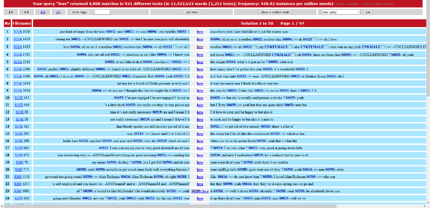
138

Figure 17. Concordance lines for the simple query ‘love’ in the Spoken BNC2014.

139

The usability of the Spoken BNC2014 in CQPweb was trialled extensively. Our first

opportunity to test the corpus data in the interface was the Spoken BNC2014 early access data

grant scheme. In 2016, we released a 4,789,185-word sample of Spoken BNC2014 data to a small

set of researchers who we had selected, based on an application process. This sample, known as

the Spoken BNC2014S, contained texts from the earlier stage of data collection, which had

already been transcribed and converted into XML (see McEnery et al. 2017b for more

information). The selected researchers were given exclusive early access to this sample in the

CQPweb interface for the purpose of conducting research projects, as proposed in their

applications. The benefit of the data grant scheme for the research team was the live trialling of

the corpus data in CQPweb; we encouraged the researchers to give us feedback about the corpus

data and the tool itself. The benefit for the researchers was exclusive early access to the corpus,

as well as the opportunity to publish their research in either a special issue of the International

Journal of Corpus Linguistics (McEnery et al. 2017a), which includes the official citation paper for

the corpus (Love et al. 2017a), or a book in the Routledge Advances in Corpus Linguistics series

(Brezina et al. forthcoming). The data grant researchers, and their research topics, are listed

below.

• International Journal of Corpus Linguistics special issue (McEnery et al. 2017a)

o Robert Fuchs (intensifiers)

o Jacqueline Laws, Chris Ryder and Sylvia Jaworska (verb-forming suffixation)

o Tanja Hessner and Ira Gawlitzek (intensifiers)

o Andreea S. Calude (demonstrative clefts)

• Routledge Advances in Corpus Linguistics book (Brezina et al. forthcoming)

o Jonathan Culpeper and Mathew Gillings (politeness)

o Karin Aijmer (intensifiers)

o Karin Axelsson (tag questions)

o Deanna Wong and Haidee Kruger (backchannels)

o Tanja Säily, Victorina González-Díaz, and Jukka Suomela (adjective comparison)

o Gard Jenset, Barbara McGillivray and Michael Rundell (dative alternation)

o Andrew Caines, Michael McCarthy and Paula Buttery (zero auxiliary

progressives)

o Laura Paterson (untriggered reflexive pronouns)

140

The feedback I gathered from these researchers was extremely useful in the further development

of the Spoken BNC2014, as we approached the full public release of the corpus in September

2017. We had, for example, proposed a new age categorisation scheme, which we intend to allow

a more sophisticated analysis of age grading than offered by the Spoken BNC1994 (see Section

3.3.5, p. 49). What we had failed to consider was the importance of comparing the Spoken

BNC2014 data to its predecessor according the same age groups, and the two schemes were not

fully compatible. Based on feedback from the data grant authors about this problem, I

categorized the Spoken BNC2014 speaker metadata according to both the old and new age

schemes, and both are offered in the full release.

Another issue which was drawn to our attention was the possibility that some features

(e.g. tag questions) had not been consistently transcribed. Although we were aware of the issue

of inter-transcriber inconsistency (see previous chapter), we had not thought of a way of

facilitating the exploration of this in the corpus. It was suggested by data grant authors that we

include a code for the transcriber of each audio recording in the metadata of the equivalent

corpus texts. Having done this, it is now possible to compare the search results in the corpus

according to who transcribed it, and explore possible variation.

A final example is a request to facilitate the creation of subcorpora according to text

metadata categories which are non-standardised free-text, and therefore not searchable in

restricted query mode (e.g. inter-speaker relationship, recording location and topics covered).

This is now possible in the ‘Create and edit subcorpora’ menu of the final release in CQPweb.

Once the remaining corpus texts (i.e. those processed after the release of the Spoken

BNC2014S) were ready, and the entire corpus indexed into CQPweb, Andrew Hardie and I

organised a workshop at the International Corpus Linguistics Conference (2017),

which was

hosted by the University of Birmingham and took place in July 2017 – two months before the

public release of the corpus. Here, participants were granted temporary access to the entire

corpus in CQPweb, and I gathered feedback which, like that of the early access data grant

researchers, could be taken into account in advance of the public release. One example of such

feedback was a request for the facility to conduct keyword analysis between the Spoken

BNC2014 and other corpora, including the BNC1994 (XML edition). Like the data grant

feedback, we were able to implement most reasonable requests made in the feedback.

http://www.birmingham.ac.uk/research/activity/corpus/events/2017/cl2017/pre-conference-workshop-9.aspx

(last accessed September 2017).

141 
 
  As  mentioned,  the  Spoken  BNC2014  was  publicly  released  via  CQPweb  on  25 
September 2017, along with a user guide (Love et al. 2017b), which provides information about 
the corpus make-up as well as the functionality of the CQPweb interface. 
 
6.5  Chapter summary 
In this chapter, I have described three important stages in the construction of the Spoken 
BNC2014 – conversion into XML, automatic annotation and corpus dissemination.  
With regards to the conversion of the corpus transcripts into XML (Section 6.2), I have 
shown  how  the  transcription  scheme  (Appendix  J,  p.  224)  was  designed  specifically  with 
automatic  mapping  to  XML  in  mind,  and  how  a  PHP  script  was  set  up  to  facilitate  this 
automated  process.  I  showed  that,  despite  this  intention,  many  and  various  errors  in  the 
transcription codes were detected by the script, and that the script proved to be crucial in the 
process of quality control.  
  In  the  section  on  annotation  (Section  6.3),  I  introduced  the  CLAWS  tagger  (Garside 
1987) and justified our decision to use the lesser-known set of resources available for the tagger 
–  the  spoken  resources  (Garside  1995).  Despite  its  age,  the  spoken-trained  CLAWS  tagger 
appears  to  perform  much  better  on  the  Spoken  BNC2014  data  compared  to  the  standard 
(written)  tagger  –  achieving an  error  rate  of  2.5%  compared  to  7.3%  for the  standard  tagger 
resources. I also introduced the USAS tagset for semantic categories (Rayson et al. 2004), which 
we used for semantic annotation of the corpus. 
  Finally,  I  discussed  our  procedure  for  releasing  the  corpus  publicly.  The  Spoken 
BNC2014 was made available publicly (and for free) via the CQPweb platform (Hardie 2012) in 
September 2017. Before this, though,  we were able to trial  its use  in real research settings  by 
releasing the Spoken BNC2014S to a small set of selected researchers in 2016. This, and other 
trialling methods, was described. The Spoken BNC2014 XML files and metadata will be available 
for free public download as of Autumn 2018. 
  With  the  research,  design and  compilation  of  the  Spoken  BNC2014  accounted for in 
Chapters 2 to 6, the final aim of this thesis is to demonstrate how the corpus may be used in 
linguistic  research.  In  the  next  chapter,  I  compare  the  Spoken  BNC2014S  with  the  Spoken 
BNC1994DS with regards to the occurrence of bad language. 

 
142 
 
7         Analysing the Spoken BNC2014 
7.1  Introduction 
This thesis has, thus far, documented the main stages of the compilation of the Spoken 
BNC2014. It is now time to demonstrate how the corpus may be used for linguistic research. 
This  chapter  aims  to  investigate  bad  language  in  present-day  spoken  British  English,  with 
comparison to that of the 1990s, by comparing two corpus sampling points of spoken British 
English collected in the 1990s and 2010s. I report on the analysis of bad language words (BLWs) 
in  the  early  sample  version  of  the  Spoken  BNC2014,  making  comparison  to  the 
demographically-sampled component of the Spoken BNC1994. The structure of this chapter is 
necessarily uncharacteristic of the chapters which have preceded it, as this is very much a self-
contained piece of analysis, built upon the dataset I have constructed. In Section 7.2, I present a 
literature  review  which  explores  the  background  of  swearing  as  an  object  of  study,  before 
discussing various linguistic definitions of swearing and laying out the work of McEnery (2005), 
which is most influential to this study. Section 7.3 presents the methodology and data used in 
this chapter, and Section 7.4 presents the findings as a series of case studies, which are informed 
by literature on specific aspects of swearing in spoken British English. The case studies aim to 
address the following research questions: 
 
RQ1. (How) does the overall frequency of BLW occurrence differ between the corpora? 
(Section 7.4.1) 
RQ2. (How) does the distribution of BLW strength differ between the corpora? (Section 
7.4.2) 
RQ3.  (How)  does  the  social  distribution  of  a  sample  of  BLWs  differ  between  the 
corpora? (Sections 7.4.3 to 7.4.5) 
RQ4.  Using  FUCK  as  an  appropriate  case  study,  what  can  manual  annotation  of  the 
‘category of insult’ reveal about possible differences in the meaning of this BLW between 
the two corpora? (Section 7.4.6) 
 
RQs  1  and  2  aim  to  establish  a  bird’s  eye  view  of  the  BLW  landscape,  focussing  on  notable 
differences  between  the  Spoken  BNC1994DS  and  the  Spoken  BNC2014S.  RQs  3  and  4  are 

143

more focussed, as necessitated by the limited scope allowed within this single chapter. Findings

are presented throughout these sections, and then summarised in the conclusion (Section 7.5),

which also includes a consideration of the limitations of this work.

As a whole, this chapter does not purport to produce a full analysis of all bad language in

the two Spoken British National Corpora. Such an aim is beyond the scope of this thesis. Rather,

it aims to point towards some initial findings about changes in BLW use between the two

corpora which may encourage further research in the future while, crucially, demonstrating some

of the features and uses of the Spoken BNC2014.

7.2 Swearing in linguistics

7.2.1 Swearing as an object of study

Swearing is “a rich emotional, psychological, and sociocultural phenomenon” (Jay 2009a:

153). Although swearing, and societal discourse around swearing, has existed for centuries, it has

only started to become a prominent subject of research in linguistics, psycholinguistics,

neurolinguistics, history and other disciplines, since the 1960s (Partridge 1947, Montagu 1967,

1973, Lakoff 1975, Cheshire 1982, Andersson & Trudgill 1992, Hughes 1998, van Lancker &

Cummings 1999, McEnery 2005, Ljung 2011, Lutzky & Kehoe 2015). Ljung (2011: 4) claims that

many previous studies into swearing “are not intended as overall accounts of swearing but focus

on particular aspects of swearing that they find interesting”, rendering it difficult to link together

the various studies coherently. Although the work in this chapter does not aim to unify all

existing scholarship about swearing across disciplines and varieties, it does, on the other hand,

aim to act as a starting point for the overall understanding of swearing in contemporary spoken

British English. It sets out to investigate how the “passing parade of words that constitute bad

language” (McEnery 2005: 2) has changed in recent spoken British English. Clearly such an aim

requires an empirical approach (unlike the approach of many of the earlier studies cited above),

and corpus linguistics has been shown comparatively recently to facilitate the sophisticated

analysis of swearing in a range of datasets (Rayson et al. 1997, McEnery et al. 1999, 2000,

McEnery & Xiao 2004, McEnery 2005, Stenström 2006, Thelwall 2008, Di Cristofaro 2014,

Drange et al. 2014, Ebeling & Ebeling 2014, Lutzky & Kehoe 2015). In the context of the

Spoken BNC2014, and with a view to demonstrating some of the ways in which it can be

employed, swearing is an appropriate avenue of enquiry, because it is a “marker of distinction in

English” (McEnery 2005: 24); observing variation in the use of swearing across demographic

groups, as can be afforded by the Spoken BNC2014, can lead to conclusions which may support

or challenge existing ideas about so-called prestigious language. Clearly, then, in terms of

144

similarity to previous studies, it is Chapter 2 of McEnery (2005) that is most relevant: an analysis

of swearing in a dataset derived from the demographically-sampled component of the Spoken

BNC1994 (henceforth Spoken BNC1994DS). What follows is a review of literature sufficient to

lay the groundwork for the present study. It addresses the issue of how swearing should be

defined in a corpus linguistic study, and discusses the approach of McEnery (2005, Chapter 2).

More specific literature, relating to the strength and the quantitative and qualitative distribution

of swearing in contemporary spoken British English, is introduced in relevant sections of

analysis.

7.2.2 Defining swearing

Although “there is more to being impolite than just swearing” (Culpeper 2011: 6), it is

fair to say that taboo words form the portion of a given language that is most strongly associated

with causing offence. Stone et al. (2015: 66), in their review of literature on swearing in western

health settings, offer a set of explicit criteria for identifying swearing:

1. Refer to something that is taboo, offensive, impolite, or forbidden in the culture;

2. Can be used to express strong emotions, most usually of anger;

3. May evoke strong emotions, most usually of anger or anxiety;

4. Include the strongest and most offensive words in a culture—stronger than slang and

colloquial language; and

5. May also be used in a humorous way and can be a marker of group identity.

The terms used to discuss swearing in the literature vary, depending upon the definitions to

which individual authors subscribe; these definitions can be separated superficially into two

camps. Firstly, there are those who adopt a broad approach to swearing and include all types and

instances of words which may cause offence. Jay (2009a: 153), in his review of research on taboo

words, describes the “lexicon of offensive emotional language” using the terms taboo words and

swear words interchangeably. For him, these are words which are “sanctioned or restricted on both

institutional and individual levels under the assumption that some harm will occur if…spoken”

(Jay 2009a: 153). Stone et al. (2015) use the term swearing, and their criteria (above) clearly include

any word which is used to cause offence. McEnery (2005), in his corpus study of swearing in

1990s spoken British English, also uses swearing/swear words, but only as a sub-category of bad

language words (BLWs). BLWs can be split into two types: (a) literal and non-literal use of words

which would canonically be described as swear words (e.g. SHIT, FUCK); and (b) other words

145

which may be used “to cause offence” (McEnery 2005: 2), but which would not be considered

swear words otherwise (e.g. PIG, TART). The distinction between “swear words and terms of

abuse” (McEnery et al. 2000: 37) described here has roots in Hughes (1998), which was a starting

point for McEnery’s work (i.e. McEnery et al. 1999).

The other camp comprises those who, unlike Jay (2009a), Stone et al. (2015) and

McEnery (2005; et al. 2000), take a narrow approach, and exclude certain potentially offensive

words from their definition of swearing. Ljung (2011: viii), in his cross-linguistic study into the

“shape, use and manifestations” of swearing, defines bad language via a typology that has much

in common with McEnery (2005) but, crucially, excludes literal uses of swear words. He asserts

that swear words are exclusively emotive in meaning rather than referential, to the extent that

“taboo words with literal meaning cannot be regarded as swearing” (Ljung 2011: 12). The reason

posited is that taboo words, when used in their literal/non-taboo sense, can be replaced by other

non-taboo synonyms (e.g. we fucked can be replaced by we bonked), but that the same word used in

a taboo sense cannot be replaced by the same set of synonyms (i.e. *bonk you is not a suitable

replacement for fuck you). This view is shared by Lutzky and Kehoe (2015: 167), who do use the

term swearing but “do not regard literal uses of taboo words as swearing (e.g. the word shit being

used with reference to the excretory system)” – the reason being that literal uses are said not to

“express emotions”.

In this chapter, I adopt the broad approach to swearing, specifically that of McEnery

(2005), and so henceforth use his terminology. There are two reasons for this. Firstly, it would be

difficult to replicate McEnery’s methods or compare the findings presented in this work to those

of McEnery without also applying the same selection criteria for BLWs. The second reason is

that the narrow view of bad language is flawed, because it ignores evidence about the arousing

autonomic properties of these words. It is known that swear words (i.e. the sub-category of

BLWs which are considered exclusively taboo, and are not polysemous with non-taboo uses, e.g.

FUCK, SHIT, CUNT) – encountered out of any context which would dictate whether they are

being used literally or emotively – are more psychologically arousing than non-taboo words

(Janschewitz 2008). Consequently, speakers are so-conditioned that taboo words are inherently

more memorable than non-taboo words (Jay et al. 2008) – again, when encountered out of

semantic context. Therefore, it is difficult to accept the view that swear words (e.g. SHIT)

somehow do not trigger such automatic responses when used literally (e.g. to refer to the act of

defecating), and yet do trigger psychological arousal when used emotively (e.g. as an interjection).

I adopt the view that it is the form of the swear word that inherently carries the status of taboo, as

is socially conditioned, and that literal uses of such words should still be considered valid

146

examples of bad language. This is, in fact, what distinguishes swear words as a type of BLW

from McEnery’s (2005) other type of BLW: words which are not swear words in and of

themselves, but which could be used to cause offence.

7.2.3 McEnery’s approach to bad language

As stated, the aim of this chapter is to use the Spoken BNC2014S to replicate the work

of McEnery (2005), who studied bad language in the Spoken BNC1994DS. McEnery (2005)

includes a chapter devoted to the analysis of BLWs in a specially curated subset of the Spoken

BNC1994DS known as the Lancaster Corpus of Abuse (LCA); the construction of the LCA is

detailed by McEnery et al. (1999, 2000). In short, the LCA is a corpus comprised only of

instances of bad language (and appropriate context on either side of each instance to understand

their use). In addition to quantitative analysis of the distribution of the BLWs across the

sociolinguistic categories of gender, age and socio-economic status, McEnery (2005) conducts

qualitative analysis of each BLW, using a bespoke bad language categorization scheme (Table 20,

overleaf),

finding that “the use or lack of use of BLWs is a fault line along which age, sex and

social class may be differentiated” (McEnery 2005: 50). Although McEnery (2005: 27) concedes

that the categories of insult (Table 21, overleaf) are “certainly susceptible to further

development”, he shows that they “seem at least to display discriminating power” (McEnery

2005: 28) – finding, for example, that males significantly prefer ‘EmphAdv’ and ‘AdvB’ BLWs,

whereas females significantly prefer ‘Gen’, ‘PremNeg’ and ‘Idiom’ BLWs (p. 31). Despite this,

the LCA annotation has received criticism. Ljung (2011: 28) criticises several of the categories of

McEnery’s categorization scheme, including ‘Idiom’, ‘Image’ and ‘Pron’, suggesting that the

scheme ought to be used with caution.

The categorization scheme was created alongside the LCA itself, and its development is also described by

McEnery et al. (1999, 2000).

147

Table 20. LCA annotation scheme (McEnery 2005: 27); modifications are italicised.

Field

Feature marked

Possible values

Gender of speaker

M = male, F = female, X = unknown

Social class of speaker

As per social class categories of BNC (see Aston &

Burnard 1998)

Age of speaker

As per age categories of the Spoken BNC1994DS (see

Aston & Burnard 1998)

Category of insult

As per Table 21.

Gender of hearer

As per gender of speaker

Person of target

1 = first person, 2 = second person, 3 = third person, X

= unknown

Metalinguistic usage

0 = no, 1 = yes

Animacy of target

+ = animate, - = non-animate, X = unknown

Gender of target

As per gender of speaker

Number of target

1 = singular, 2 = plural, X = unknown

Quotation

Q = quotation, N = non-quotation, X = unknown

Table 21. Categories of insult in the LCA annotation scheme (McEnery 2005: 27).

Letter

Code

Description

PredNeg

Predicative negative adjective: ‘the film is shit’

AdvB

Adverbial booster: ‘Fucking marvellous’ ‘Fucking awful’

Curse

Cursing expletive: ‘Fuck You!/Me!/Him!/It!’

Dest

Destinational usage: ‘Fuck off!’ ‘He fucked off’

EmphAdv

Emphatic adverb/adjective: ‘He fucking did it’ ‘in the fucking car’

Figurtv

Figurative extension of literal meaning: ‘to fuck about’

Gen

General expletive ‘(Oh) Fuck!’

Idiom

Idiomatic ‘set phrase’: ‘fuck all’ ‘give a fuck’

Literal

Literal usage denoting taboo referent: ‘We fucked’

Image

Imagery based on literal meaning: ‘kick shit out of’

PremNeg

Premodifying intensifying negative adjective: ‘the fucking idiot’

Pron

‘Pronominal’ form with undefined referent: ‘got shit to do’

Personal

Personal insult referring to defined entity: ‘You fuck!’/‘That fuck’

Reclaimed

‘Reclaimed’ usage—no negative intent, e.g. Niggers/Niggaz as used by

African American rappers

148

Oath

Religious oath used for emphasis: ‘by God’

Unc

Unclassifiable due to insufficient context

7.3 Method

7.3.1 Methodological procedure

The aim of this work is to replicate McEnery (2005) by analyzing a large set of BLWs in

the Spoken BNC2014S and comparing their frequency, sociolinguistic distribution and use to

that of the Spoken BNC1994DS, commenting on any indications of changes in bad language

over the last twenty years. McEnery (2005: 30) lists a set of forty-nine BLWs, which was the

object of his study. These are:

arse, arsehole, balls, bastard, bird, bitch, bloody, bollocks, bugger, Christ, cow, crap, cunt,

damn, dickhead, fuck, gay, git, god, hell, hussy, idiot, jesus, jew, moron, motherfucker,

nigger, paki, pig, pillock, piss, pissed off, poofter, prick, screw, shag, shit, slag, slut, sod,

son-of-a-bitch, spastic, tart, tit, tits, tosser, twat, wanker, whore

For this study, using only this set of BLWs would be insufficient; I had to take into account the

possibility of new BLWs having emerged since the early 1990s. Therefore, I extended the original

list of BLWs by adding those from two other sources. The first set is those that were included by

the UK’s Office of Communications (Ofcom), which recently published a guide to offensive

language in broadcast media (Ofcom 2016). This greatly extended McEnery’s original list, adding

the following BLWs:

batty boy, beaver, beef curtains, bellend, bender, bint, bloodclaat, bonk, bukkake,

bullshit, bum boy, bumclat, bummer, chi-chi man, chick with a dick, chinky, choc ice,

clunge, cock, cocksucker, coffin dodger, coloured, coon, cretin, cripple, dago, darky, dick,

dildo, div, dyke, faggot, fairy, fanny, feck/effing, fenian, flaps, fop (fucking old person),

fudge-packer, gash, gender bender, ginger, gippo, goddam, golliwog, gook, he-she, ho,

homo, honky, hun, jap, jesus christ, jizz, jock, kafir/kufaar, kike*, knob, kraut,

lezza/lesbo, loony, mental, midget, minge, minger, mong, muff diver, munter, nancy,

nazi, negro, nig-nog, nonce, nutter, old bag, pansy, papist, pikey, pissed / pissed off,

polack, poof, prickteaser, prod, psycho, punani, pussy, queer, raghead, rapey, retard,

rugmuncher/ carpetmuncher, sambo, schizo, shirt lifter, skank, slapper, slope, snatch,

149

sod-off, son of a bitch, spade, spastic/spakka/spaz, special, spic, taff, taig, tranny,

vegetable, window licker, wog, wop

The second source is the set developed by Lutzky and Kehoe (2015), in their analysis of bad

language in computer-mediated communication. While some of their search terms, such as omg

(oh my God) and ffs (for fuck’s sake), are unsurprisingly informed by research on computer-mediated

communication rather than speech (e.g. Thelwall 2008), others which do not appear in either the

lists of McEnery (2005) or Ofcom (2016) (e.g. douche, jerk, wank) do, by intuition, appear to be

good candidates for BLW status in 2010s spoken British English. The full list of additional

words offered by Lutzky and Kehoe reads:

bimbo, bollock, boob, butt, chav, dork, douche, dumb, fag, fart, fatass, ffs, imbecile, jeez,

jerk, omg, pimp, prat, sonofabitch, suck, swine, turd, wank, wtf, wuss

The use of both the Ofcom (2016) guide and Lutzky and Kehoe’s (2015) work as a basis for

extending McEnery’s original list resulted in a new set of 173 BLWs (see Appendix Q, p. 264, for

the master list of BLWs used in this study and the syntax used to search for them). In several

cases, I was motivated to merge separate words which I prefer to treat as morphological variants

of the same lemma. Some of the extra words that were derived from the two sources (as listed

above) did not actually create an entirely new BLW entry on my new list, but rather served as

additional morphological variants not necessarily captured by McEnery (2005). For example,

McEnery (2005) includes bollocks but not bollock; I added the singular form to the search query as

a morphological variant of the lemma BOLLOCK, rather than treating it as a separate BLW entry.

McEnery’s wanker was merged with Lutzky and Kehoe’s wank in the same vein, under the lemma

WANK. Likewise, Ofcom (2016) lists sod and sod off as separate entries, but I have merged these

under the lemma SOD; dick and dickhead are now merged under the lemma DICK; and god and

goddam are now merged under the lemma GOD. For the sake of consistency with this decision I

then merged some of McEnery’s (2005) original BLWs: piss and pissed off under the lemma PISS; tit

and tits under the lemma TIT; and arse and arsehole under the lemma ARSE.

The next step was to create suitable search queries for each of the BLWs under

investigation. I used CQP syntax to refine the queries for precision, and originally planned to use

lemma searches for BLWs which were clearly morphological headwords (e.g. CRAP). This would

simplify the search queries and ensure that no rare morphological variants were omitted from the

search (i.e. maximizing recall). However, the automatic lemmatization of the corpus data was not

150

reliable enough to do this; the lemma search for CRAP ([lemma="crap"%c]), for example, retrieved

289 instances comprising crap, crapped, crapping, crappest and crapper, but the non-lemma search

([word="crap.*"%c]) retrieved 321 matches, including relevant forms like crappy, crapper and crapola

which were not detected by lemmatization. This observation forced me to abandon searching for

lemma forms and adapt the search queries accordingly.

Once the appropriate search queries were written, I was then able to conduct strength,

frequency, distribution and manual analyses of the BLWs as per the following analytical

procedure:

(1) Search in the Spoken BNC1994DS and Spoken BNC2014S for each BLW in turn;

(2) Observe BLWs which have a frequency of zero in both corpora and eliminate from

further analysis;

(3) Analyse the strength of BLW use between the two corpora;

(4) Analyse BLWs which have changed in relative frequency to the greatest extent between

the two corpora;

(5) Demographic distribution: select some of the most commonly occurring BLWs in both

corpora, and analyse their frequency per speaker metadata category according to gender,

age and socio-economic status;

(6) Annotate and analyse the BLW FUCK according to the LCA annotation scheme’s

‘categories of insult’ (McEnery 2005).

Steps 1-5 were carried out by making the queries in both corpora in CQPweb (Hardie 2012) and

recording the frequencies in a spreadsheet. For step 3, I compared the sum of instances of each

BLW according to each ranking of strength as assigned by Ofcom (2016), as discussed in Section

7.4.2. For step 4, significance (log-likelihood) and effect size (log ratio, see Hardie 2014a) of the

differences in frequency across the corpora were calculated (for the frequency analysis) using the

UCREL Log-likelihood and effect size calculator.

For step 5, I must make explicit my use of

terminology: I use the term ‘demographic category’ or simply ‘category’ to identify types of

speakers collated according to the three relevant demographic identities gender, age and socio-

economic status (so, age is an example of a category). For the subsections within each category (e.g.

age 15-24) I use the term ‘demographic group’ or ‘group’. Again, the UCREL calculator was used

to ascertain significance and effect size for diachronic comparisons of individual groups (e.g.

differences between 1990s females and 2010s females), while the UCREL Significance Test

http://ucrel.lancs.ac.uk/llwizard.html (last accessed September 2017).

151

System

was used to calculate the log-likelihood of the synchronic differences within categories

(e.g. differences between age groups in the 1990s). The selection of BLWs for treatment in step 5

was motivated by frequency; comparison across demographic groups would be most effective

for relatively high frequency BLWs. For step 6, I downloaded the relevant concordance lines for

both corpora and analysed random samples of 1,000 of each of them according to the LCA

annotation scheme’s categories of insult in a spreadsheet.

7.3.2 Data

In this section, I briefly describe the corpora under investigation before turning attention

to two methodological issues worth discussing: the comparability of the 1994 and 2014 corpora,

and attributing findings to language change.

This study compares the spoken components of both British National Corpora. Both

corpora were accessed via Lancaster University’s CQPweb server (Hardie 2012). The

demographically-sampled component of the Spoken BNC1994 (hereafter Spoken BNC1994DS)

contains 5,014,655 tokens across 153 texts, while the Spoken BNC2014 Sample (hereafter

Spoken BNC2014S) contains 4,789,185 tokens across 567 texts. As mentioned in Section 6.4 (p.

136), the Spoken BNC2014S is a subset of the Spoken BNC2014 which was released exclusively

to selected researchers in 2016, while the rest of the corpus was still being compiled (see

McEnery et al. 2017b). The corpus texts were transcribed from recordings collected between

2012 and 2015.

Table 22 (overleaf) summarises the token counts for each demographic group in both

corpora. Given that there are a certain number of ‘unknown’ speakers in each demographic

category in both corpora, the sum of analysable groups (i.e. all groups excluding ‘unknown’)

within each category does not equal the sum of tokens in the given corpus. For example, as

described in Section 3.3.5 (p. 49), the comparison of speaker age between the two Spoken British

National Corpora does require that some speakers are placed into the ‘Unknown’ age group

despite having some information about their age. This explains why, for example, the sum of

Spoken BNC2014S tokens analysed in the following age sections (3,535,521) is considerably

lower than the sum of tokens in the Spoken BNC2014S (4,789,185).

http://corpora.lancs.ac.uk/sigtest/ (last accessed September 2017).

152

Table 22. Token counts for the groups within demographic categories gender, age and socio-

economic status in the Spoken BNC1994DS and Spoken BNC2014S.

Demographic category

Group

Tokens in group

Spoken BNC1994DS

Spoken BNC2014S

Gender

Female

2,662,805

2,872,758

Male

1,726,993

1,911,836

TOTAL

4,389,798

4,784,594

Age

0-14

435,286

69,362

15-24

596,113

957,924

25-34

816,024

395,679

35-44

825,857

656,501

45-59

859,736

527,901

60+

783,594

928,154

TOTAL

4,316,610

3,535,521

Socio-economic status

852,100

2,641,196

924,336

622,858

842,149

93,004

485,276

1,401,946

TOTAL

3,103,861

4,759,004

In terms of the comparability of these corpora, it could be argued that, since neither of

the Spoken British National Corpora were sampled with the explicit aim of studying BLWs, it is

difficult to claim that the sampling conditions allowed for a comparable amount of BLW use.

However, it can firstly be assumed that the Spoken BNC1994 facilitated the natural occurrence

of BLWs, given its surreptitious approach to recording (Crowdy 1993: 260). Secondly, as

explained in Section 3.4.3 (p. 70), the aim of the Spoken BNC2014 team was to facilitate the

recording of conversations in a way which minimized intrusiveness beyond what was required of

ethics procedures introduced since the compilation of its predecessor. Although the requirement

for informed consent of all speakers prior to the commencement of recording does mean that

the contexts of recording are not identical, it does not seem to be the case that speakers were

inhibited from speaking naturally. Harry Strawson, a Spoken BNC2014 contributor who

submitted over a dozen recordings,

claimed that “it was surprising how quickly people seemed

to forget they were being recorded” (Strawson 2017: 41). Furthermore, contributor interviews

(see Section 3.2.6, p. 33) seemed to support this claim:

Strawson had been guaranteed anonymity as per the standard contract made between the Spoken BNC2014

research team and all contributors. However, since his article was published I understood there to be no issue with

mentioning him by name here.

153

3: You didn’t completely forget because it was right there in front of you on the

table, but there would be times where, one of them in particular where we were playing a

game, where we forgot and somebody said oh yes I forgot we were recording this or are we still

recording? Or something like that. (Appendix A, p. 208)

9: …I forgot about it straight away.

8: I think people forgot about it after the first couple of minutes. (Appendix B, p.

211)

Finally, with specific reference to bad language use, while McEnery et al. (1999: 51) do state that

the observer effect may reduce the quantity of BLW usage, they “see no reason to believe that

the patterns of usage for individual [bad language] words are affected by this observer effect”

(emphasis added).

Another issue is the relationship between the comparison of two corpora and claims

about diachronic language change. In this chapter, I am clearly interested in change over time;

this interest is the primary motivating factor of this investigation. However, I am only able to

compare two sampling points – the early 1990s and the 2010s. When making such comparisons

in terms of, for example, the frequency of BLWs, the possible outcomes are necessarily limited

to three patterns: one may observe an increase between point A and point B, or a decrease, or

stability (cf. ‘lockwords’, Baker 2011). Without comparable data, taken from a larger number of

sampling points, it is impossible to conclude whether an observed change or stasis represents,

for example, part of a long-existing development, or, on the other hand, a short-term

phenomenon

- a bump in the linguistic road.

In terms of comparative work between the first and second of the British National

Corpora, this is a limitation which cannot be avoided by virtue of having available data from only

two sampling points; the Spoken BNC2014 represents only the second sampling point of its

type. To create more comparable sampling points, one has two options. One method is to collect

data from the past (see e.g. the creation of a 1930s LOB corpus, Leech & Smith 2005). An older

Spoken BNC of a comparable point in time would need to contain data from the 1970s;

although some recordings of casual conversations from this time likely do exist, it is not a

reasonable aim to curate a 10-million-word corpus, of a range of UK regions and sociolinguistic

groups, from this decade. The further back through the 20

century one looks, the harder this

Although advanced statistical procedures can be applied which can assess the confidence with which

generalisations can be made about such two-point comparisons (Brezina forthcoming).

154

task becomes. The other option is to halt comparative research into the two Spoken British

National Corpora until a third becomes available. A third comparable sampling point would be

the 2030s. It is clearly unreasonable to wait so long to conduct such research. Rather, my

approach is to compare the two corpora, make tentative comments about difference and stasis,

and insist that these research questions are revisited in the future when more data becomes

available. Therefore, I frame the findings presented in this chapter with the point in mind that

they are not alone directly indicative of language change (or stasis) per se, but rather suggestive

of change or stasis.

7.4 Results

7.4.1 Frequency comparison

The full, unfiltered

frequency list of the BLWs under investigation is provided in

Appendix R (p. 272). In total, there are 31,423 instances of (potential) BLWs identified in both

corpora (17,215 in the Spoken BNC1994DS and 14,208 in the Spoken BNC2014S). 32 of the

BLW queries, however, returned a frequency of zero in both corpora. These are:

BATTY BOY, BEEF CURTAINS, BLOODCLAAT, BUKKAKE, BUM BOY, BUMCLAT, CHI-CHI

MAN, CHICK WITH A DICK, COCKSUCKER, COFFIN DODGER, COON, DAGO, FATASS,

FENIAN, FFS, FUDGE-PACKER, KAFIR/KUFAAR, KIKE, KRAUT, LEZZA/LESBO, MUFF

DIVER, OMG, PRICKTEASER, PUNANI, RAGMUNCHER/CARPETMUNCHER, SCHIZO,

SHIRT LIFTER, SPIC, TAIG, WINDOW LICKER, WTF

With the exception of FATASS, FFS, OMG and WTF (which derived from the Lutzky & Kehoe,

2015 list), these BLWs were taken from the Ofcom (2016) list. Many of these are described by

Ofcom as having “low recognition” among focus group participants, and several, including

BLOODCLAAT, BUKKAKE, FENIAN and KIKE, were labelled as having been identified by less than

40% of participants in an online survey of the words. Based on this, it is perhaps unsurprising

that they do not occur in the corpora. Clearly these words do exist in (at least some

variety/varieties of) British English, but they are so relatively infrequent that one of two

approaches would be required to access them: either (a) a much larger general corpus or (b)

specialised corpora which would be gathered based upon knowledge of where these words are

most likely to be spoken.

With these BLWs eliminated, 141 (potential) BLWs remain which occur at least once in

The frequencies are the total number of hits produced by each query, regardless of precision. Non-BLW uses of

the search terms, if present (due to polysemy), have not been identified or removed from the frequency results.

155

either of the corpora (see Appendix R, p. 272), which includes figures for percentage change,

significance and effect size. Overall, the total sum of these BLWs in both corpora suggests a fall

in the use of bad language between the 1990s and 2010s – falling from 3,433 per million (1990s)

to 2,967 per million (2010s) which is significant at the p<0.0001 level with a log ratio of 0.21.

Despite the significant decrease in BLW occurrence, in the context of previous research this

does not seem alarming; these frequencies roughly correspond with Jay (2009b: 90), who

reviewed several empirical studies into bad language and reported that swearing constitutes 0.3 to

0.7% of speakers’ output. Therefore, it would be difficult to claim that the difference in

frequency between the corpora is suggestive of some wider decline in the use of BLWs among

British English speakers. More likely is the difference in speaker awareness that they were being

recorded, as discussed in Section 3.3.3 (p. 41) – perhaps the Spoken BNC2014S speakers, who

were aware of the recordings taking place, were slightly less likely to use bad language as often as

their Spoken BNC1994DS predecessors, who were mostly unaware (see also McEnery et al.

1999: 51).

What is perhaps harder to attribute to speaker awareness is the strength of the BLWs

which speakers do produce, which is the focus of the next section.

7.4.2 Strength

An area of interest with regards to bad language is the strength of BLWs. The strength,

or potential offensiveness, of BLWs has been shown to vary according to social context; the

same BLWs may be used for offensive purposes such as blasphemy, hate speech or abuse, but

also to achieve “positive social outcomes”, e.g. through humour, sex talk or in-group slang (Jay

2009a: 155). This is especially true for what Jay calls ‘conversational swearing’ – the type of BLW

use studied by McEnery (2005) and in the present chapter. Jay’s view is that “there is no

evidence of harm from fleeting expletives or from conversational or cathartic swearing” (2009b:

93). Despite this, it is clear that some BLWs are considered less acceptable than others, even in

informal, familial conversation such as that in the Spoken British National Corpora. There is

evidence, for example, that the strength of bad language exerts some control on cognition.

Bowers and Pleydell-Pearce (2011) analysed electrodermal activity in participants reading aloud

the words fuck and cunt, and their euphemistic equivalents f-word and c-word, and found that

“people find it more stressful to say aloud a swear word than its corresponding euphemism”

(Bowers & Pleydell-Pearce 2011: 4). Furthermore, males are said to be genetically predisposed to

produce stronger BLWs more than females, due to evolutionary intergroup aggression among

males (Güvendir 2015).

156

It is also the case that the relative strength of BLWs is a metalinguistic topic that is salient

in the public consciousness (Dawaele 2015); speakers are usually able to make clear judgements

about the strength or offensiveness of bad language words – although, out of context, it is

difficult to predict these perceptions based solely on the linguistic unit (Young 2004). Such

evaluations are nonetheless used to inform broadcasting practices with regards to the airing of

potentially offensive content, e.g. the watershed,

or the classification of films according to

audience age. Millwood-Hargrave (2000) conducted a study of public opinion of the strength of

BLWs which, along with a report by the British Board of Film Classification (BBFC), was used

by McEnery (2005: 30) to create a “scale of offence” for analysing BLWs (Table 23).

Table 23. A scale of offence (McEnery 2005: 30).

Categorisation

Words in the category

Very mild

bird, bloody, crap, damn, god, hell, hussy, idiot, pig, pillock, sod, son-of-a-bitch, tart

Mild

arse, balls, bitch, bugger, christ, cow, dickhead, git, jesus, jew, moron, pissed off, screw,

shit, slag, slut, sod, tit, tits, tosser

Moderate

arsehole, bastard, bollocks, gay, nigger, piss, paki, poofter, prick, shag, spastic, twat,

wanker, whore

Strong

fuck

Very strong

cunt, motherfucker

Using the scale of offence, McEnery (2005: 30) finds that males draw “typically from a stronger

set of words than females”, while BLW strength tends to decrease with rising age as well as

socio-economic status.

The words and their ratings in the McEnery (2005) scale do not necessarily represent

present-day BLW use. Since it seems that the BBFC no longer publishes a list of BLWs and their

perceived offensiveness (BBFC 2014: 6), I sought out a new source of updated consumer ratings.

The Ofcom (2016) report, introduced in Section 7.3.1, not only provides a present-day list of

over one-hundred-and-fifty BLWs with which further research could be undertaken, but many of

these words have been assigned a level of offensiveness according to the consumer investigations

described in the guide, which included focus groups and online questionnaires. A description of

the scale of offence used by Ofcom (2016) is provided in Table 24 (overleaf) and the words

considered are listed in Table 25 (overleaf).

The time in which adult content may be broadcast; in the UK this is between 21:00 and 05:30.

157

Table 24. Scale of offence for bad language (Ofcom 2016: 3).

Categorization

Description

mild

of little concern

medium

potentially unacceptable pre-watershed but acceptable post-watershed

strong

generally unacceptable pre-watershed but mostly acceptable post-

watershed

strongest

highly unacceptable pre-watershed, but generally acceptable post-

watershed

Table 25. BLWs in the Ofcom (2016) report, which are given unambiguous ratings in the scale

of offence.

Categorisation

Words in the category

mild

arse, bloody, bonk, bugger, cow, crap, cretin, damn, div, ginger, git, god, hun, jesus

christ, jock, loony, mental, minger, nazi, nutter, old bag, psycho, sod

medium

balls, bint, bitch, bollock, bullshit, bummer, fairy, feck/effing, fop (fucking old

person), midget, munter, pansy, pikey, piss, shag, shit, slapper, son of a bitch, special,

taff, tart, tit, vegetable

strong

bastard, beaver, bellend, bender, choc ice, clunge, cock, cripple, dick, dildo, dyke,

fanny, flaps, gash, gook, he-she, ho, homo, honky, jap, jizz, knob, minge, nancy,

negro, nonce, papist, poof, prick, prod, pussy, queer, raghead, rapey, skank, slag,

slope, slut, snatch, spade, tranny, twat, wank, whore, wop

strongest

chinky, cunt, darky, faggot, fuck, gender bender, golliwog, mong, motherfucker, nigger,

nig-nog, paki, retard, sambo, spastic, wog

Aside from better representing present-day public opinion on the strength of BLWs, the Ofcom

(2016) scheme was also applied to more than double the number of BLWs than McEnery’s

(2005), making subsequent analyses into the strength of bad language more comprehensive.

Another obvious difference between the two schemes is the number of categories; McEnery’s

(2005) scale has five while the Ofcom (2016) has only four. Although this study does not aim to

compare difference in public opinion on BLW strength between the corpus sampling points, the

mapping of one scheme onto the other is worth considering. The simplest approach is to posit

that McEnery’s (2005) ‘very mild’ and ‘mild’ categories are merged to form Ofcom’s (2016)

‘mild’ category, with McEnery’s (2005) ‘moderate’, ‘strong’ and ‘very strong’ respectively

becoming Ofcom’s (2016) ‘medium’, ‘strong’ and ‘strongest’. Doing so is minimally disruptive to

McEnery’s (2005) scheme, since the only effect is to remove the distinction between two levels

of mildness. At the stronger end of the scale, the categories can be directly compared; the

differences are perhaps suggestive of recent change in public opinion about certain BLWs. It is

notable that NIGGER, PAKI and SPASTIC are considered ‘moderate’ in McEnery (2005) but

‘strongest’ in (Ofcom 2016) – an increase of two strength levels. These are the only BLWs which

158

rose in strength to such a degree – the rest either retaining the same strength or moving up or

down by only one level.

Over 100 of the BLWs described in the Ofcom (2016) report came with ratings

according to a four-point scale of offence (Table 25). By comparing the sum of the instances of

each of these BLWs (a) at each level of the scale and (b) between corpora, an interesting

difference can be observed in the wholesale strength of BLW use (Figure 18, overleaf). In

summary:

• Mild BLWs have decreased in occurrence between the Spoken BNC1994DS and

Spoken BNC2014S (log likelihood 439.73, significant at p<0.0001).

• Medium BLWs have increased in occurrence between the Spoken BNC1994DS and

Spoken BNC2014S (log likelihood 166.55, significant at p<0.0001).

• Strong BLWs have decreased in occurrence between the Spoken BNC1994DS and

Spoken BNC2014S (log likelihood 109.13, significant at p<0.0001).

• Strongest BLWs have remained stable in occurrence between the Spoken BNC1994DS

and Spoken BNC2014S (log likelihood 1.73, not significant at p<0.05).

Figure 18. Relative frequency comparison of BLWs categorised according to the Ofcom (2016)

scale of offence.

Despite significant changes within three of the levels, the overall pattern is very similar in both

200

400

600

800

1000

1200

1400

1600

1800

mild medium strong strongest

Spoken BNC1994DS Spoken BNC2014S

159

corpora: the mild BLWs are, perhaps predictably, the most commonly uttered, and as BLW

strength increases the words occur less frequently. That is the case until the ‘strongest’ category,

which spikes up as more than twice as frequent as the ‘strong’ category in both corpora. Is it the

case that, despite the Ofcom (2016) research which in no uncertain terms reports on the high

levels of unacceptability of these words among the British general public, all 16 of the ‘strongest’

BLWs are used more than the ‘strong’ BLWs in both corpora, and almost as much as the

‘medium’ BLWs in present-day spoken British English? Looking into the data, it is clear that this

is not the case. The spike is driven by only one of the ‘strongest’ BLWs: FUCK. This accounts for

93% of all ‘strongest’ BLW occurrences in the Spoken BNC1994DS, and 96% in the Spoken

BNC2014S. In fact, it is the second most commonly occurring BLW in both corpora, second

only to BLOODY in the former and GOD in the latter, both of which are ‘mild’ BLWs (see

Appendix R, p. 272, for frequency information for all BLWs under consideration). The evidence

suggests, therefore, that FUCK – despite its apparent status as one of the strongest BLWs in

spoken British English – behaves markedly unlike its ‘strongest’ counterparts and markedly like

the weakest, and that this behaviour is unchanged between the 1990s and 2010s. This is

surprising when one considers that frequency is expected to correlate negatively with degree of

taboo (see e.g. Jay 1992). Furthermore, while each of the 16 ‘strongest’ BLWs occur at least once

in the Spoken BNC1994DS, several have a frequency of zero in the Spoken BNC2014S:

CHINKY, GENDER BENDER, GOLLIWOG, NIG-NOG and WOG. These BLWs, therefore, appear to

have fallen into obscurity in everyday British conversation; or, at least, there is not enough

language evidence in the Spoken BNC2014S for such infrequent words to occur. Another

explanation might be that these BLWs are highly referent specific; they can only be applied

felicitously to specific minority groups and thus their use could be said to reflect social context.

If a speaker does not know any East Asians, transgender people or African Americans, then such

BLWs are less likely to occur than BLWs with non-specific referents (e.g. TWAT).

The question remains as to why FUCK is so much more frequent than the other

‘strongest’ BLWs. One explanation would be that a very small group of speakers use FUCK much

more than the majority. In the Spoken BNC2014S, FUCK is uttered at least once by 116 speakers

(30.9% of all identifiable speakers), with eight speakers accounting for half of the instances of

FUCK. 260 speakers (69.1%) do not produce any instances of FUCK. Of the speakers who uttered

FUCK, the mean occurrence is 22.76 with a median of 5 and a standard deviation of 50.56.

Taking all speakers into account, including those who produced zero instances of FUCK, the

mean is 11.38, with a median of 0.5 and standard deviation of 37.60. The low mean frequencies

(relative to their standard deviations) show that a small number of speakers is using this BLW a

160

lot, and with great variation between speakers. The median of 0.5 is expected since it considers

the majority of speakers who produce FUCK zero times, but the median of 5 among only those

who do produce FUCK points towards a long tail of low-use speakers. These observations lead to

the question of whether a demographic group or groups are driving this distribution. Looking at

“how the age, sex and social class variables interact” (McEnery 2005: 45), this does appear to be

the case; the C2 socio-economic group interacts with both the female and 15-24 groups (see

Figure 19, Figure 20 and Figure 21 (overleaf) for cross-tabulated distribution graphs).

Figure 19. Gender and socio-economic status.

500

1000

1500

2000

2500

AB C1 C2 DE Unknown

Male Female

200

400

600

800

1000

1200

1400

0-14 15-24 25-34 35-44 45-59 60+ Unknown

Male Female

161

Figure 20. Gender and age.

Figure 21. Age and socio-economic status.

It should be noted that the C2 group is severely underpopulated in the Spoken BNC2014S;

perhaps too small to offer an opportunity to use FUCK, causing high relative frequencies even

with low occurrence.

Between the age and gender categories, which are generally better

populated, the distribution is skewed towards male overuse in the 15-25 group, although male

and female use is similar in the 25-34 group.

Clearly, then, FUCK appears to have a special status; it does occur very frequently,

compared to the other ‘strongest’ BLWs, but the distribution is heavily skewed. This appears to

be caused by (a) high use by a small number of individuals, and (b) a dearth of linguistic evidence

for some group combinations.

The analysis of strength has already started to reveal some large-scale changes in the

occurrence of individual BLWs over time. The following section explores how the frequency of

the BLWs varies between the two Spoken British National Corpora.

7.4.3 Change and stability in frequency

In this section, I am interested in the BLWs which differ significantly in terms of relative

frequency between the two corpora, and those which have the most similar relative frequencies.

A similar occurrence of “data sparsity” was observed by McEnery (2005: 45) while attempting to combine

demographic categories in the Spoken BNC1994.

1000

2000

3000

4000

5000

6000

7000

8000

0-14 15-24 25-34 35-44 45-59 60+ Unknown

AB C1 C2 DE

162

Of the original 173 BLWs under consideration, I have already eliminated 32 which do not occur

in either corpus, leaving 141. Starting with difference, of these 141 BLWs, 36 differ in relative

frequency between the two corpora with significance at the p<0.0001 level (LL critical value >

15.13); these are the BLWs which have either increased or decreased to the greatest extent

between the two corpora. The remaining 105 BLWs do not differ in relative frequency with

significance at the p<0.0001 level, and those with the most similar relative frequencies are

discussed later in this section.

Table 26 (overleaf) reveals the BLWs which have decreased significantly (log likelihood)

and to the greatest extent according to effect size (log ratio). Interestingly, they include some

words which are considered “strong” or “strongest” language according to Ofcom (2016):

SPASTIC, HO, CUNT, PUSSY, WANK, and BASTARD; McEnery (2005: 30), drawing upon the British

Board of Film Classification on the other hand, lists only one of these words (CUNT) as “strong”

or “very strong”, while SPASTIC, WANKER and BASTARD are considered “moderate”.

Furthermore, none of the words in Table 26 have fallen all the way to a frequency of zero,

implying that these word forms – albeit at a very low frequency in some cases (like SPASTIC or

PRAT) – are still present in spoken British English to some degree.

163

Table 26. BLWs which have decreased in use significantly (p<0.0001) between the 1990s and

2010s, ranked by effect size.

Head

Per million

(Spoken BNC1994DS)

Per million

(Spoken BNC2014S)

log-likelihood

log ratio

SPASTIC

3.8

0.2

18.97

4.18

TAFF

3.4

0.2

16.5

4.02

64.0

6.1

271.97

3.4

JOCK

4.4

0.4

18.6

3.39

PRAT

10.0

1.0

40.7

3.26

CUNT

20.5

6.7

36.09

3.07

PUSSY

18.9

2.3

72.48

3.04

SOD

39.5

6.3

130.91

2.66

BLOODY

646.7

128.2

1,846.78

2.33

BUGGER

66.4

16.3

158.84

2.03

GIT

11.8

3.3

24.28

1.82

CHRIST

50.5

15.5

95.52

1.71

FAG

25.7

9.2

39.81

1.49

WANK

17.7

8.1

17.83

1.12

BASTARD

48.1

22.6

46.06

1.09

COW

35.9

17.1

33.19

1.07

DAMN

55.8

30.3

37.65

0.88

BOLLOCK

32.1

19.0

16.62

0.76

HELL

197.0

132.6

62.01

0.57

Turning to the BLWs which have risen in use to the greatest extent (Table 27, overleaf),

an interesting picture emerges. Three of the BLWs (CHAV, DOUCHE and WUSS) have risen from

a 1990s frequency of zero; although it is impossible to claim that they did not exist at all in this

period, the data at least suggests that these BLWs have risen into more general usage in the

2010s. In terms of strength, Ofcom (2016) places only RETARD and DYKE in the “strong” or

“strongest” categories, while they are not included at all in McEnery’s scale of offense (2005: 30).

Looking at semantic categories, noteworthy is the rise of sexuality words DYKE and GAY, and

words relating to mental capacity or intellect: PSYCHO, RETARD, MENTAL and IDIOT.

Furthermore, the rise of the word NAZI is interesting – clearly this word long pre-dates the

1990s, but occurs much more frequently in the 2010s data; Ofcom (2016: 13) notes that it is

164

Table 27. BLWs which have increased in use significantly (p<0.0001) between the 1990s and

2010s, ranked by effect size.

Head

Per million

(Spoken BNC1994DS)

Per million

(Spoken BNC2014S)

log-likelihood

log ratio

CHAV

0.0

11.9

81.67

6.9

DOUCHE

0.0

4.2

28.66

5.39

WUSS

0.0

2.9

20.06

4.87

PSYCHO

0.8

7.7

32.16

3.28

NAZI

0.8

6.5

24.9

3.02

RETARD

1.4

10.6

39.74

2.93

JEW

1.0

6.9

24.39

2.79

MENTAL

9.0

61.2

214.96

2.77

JEEZ

1.4

6.3

16.48

2.17

DYKE

1.6

6.5

15.56

2.02

BOOB

6.0

23.8

56.19

1.99

GAY

9.8

33.6

68.21

1.78

BULLSHIT

3.8

12.1

22.53

1.68

SHIT

153.2

316.1

283.94

1.05

PIG

20.3

38.8

28.88

0.93

IDIOT

17.7

31.3

18.68

0.82

GOD

516.9

626.6

51.71

0.28

“mild” but “potentially offensive if used in a modern context to insult German people”.

As well as difference, it is also useful to take note of similarity, by paying attention to

what has not changed much in terms of frequency among BLWs. Of the 141 BLWs which occur

in both corpora, I have just addressed the 36 which differ at the p<0.0001 level. Eliminating

these from the present discussion leaves 105 remaining. Of these, 68 BLWs showed changes in

frequency which were not even significant at a lower LL value (p>0.05; LL critical value < 3.84).

Their relative frequencies were very similar in both corpora, and their low log ratios mean that

they can be described as ‘stable’ BLWs – or lockwords (Baker 2011). Eight of these BLWs occur

at least 100 times in both corpora. Table 28 (overleaf) shows the frequency data for these eight

BLWs. Although interesting, these BLWs do not explain themselves in terms of the reason for

their stasis; further investigation is required in order to understand how and why these words

appear to have resisted the changes which have occurred to so many of the other BLWs.

165

Table 28. BLWs which have not changed in frequency significantly (p>0.05) between the 1990s

and 2010s, and which have a minimum raw frequency of 100 in both corpora, ranked

alphabetically.

Head

Per million

(Spoken BNC1994DS)

Per million

(Spoken BNC2014S)

log-likelihood

log ratio

ARSE

43.07

45.52

0.33

0.08

BITCH

27.32

34.24

3.83

0.33

CRAP

63.41

67.03

0.49

0.08

DICK

30.51

35.91

2.16

0.24

FUCK

564.35

561.06

0.05

0.01

GINGER

35.30

35.71

0.01

0.02

JESUS

39.28

39.46

0.01

VEGETABLE

29.71

36.75

3.66

0.31

7.4.4 High-frequency BLWs: sociolinguistic distribution

So far, I have presented three categories of especially noteworthy BLWs: those which

have decreased; those which have increased; and those most commonly occurring BLWs which

remained stable. In terms of assessing similarity and difference across time periods, these

categories clearly present windows of opportunity for dictating the rest of the analysis (in similar

fashion to how keywords are used to guide the corpus-based critical discourse analyst, Baker

2006). Looking at the sociolinguistic distribution and qualitatively assessing the meanings of

these BLWs may help to answer the question of why they have changed or remained stable over

time. The stable BLWs, including the very common and well-studied FUCK (e.g. McEnery &

Xiao 2004), show no sign of growth or deterioration in terms of wholesale frequency. But as

McEnery (2005) shows with the 1990s words, bad language has a propensity for distributing

unevenly across social groups – and in terms of possible language change, the most frequent of

the stable BLWs are of interest in terms of assessing whether, if not the wholesale frequency, the

social distribution of these BLWs has changed in any way.

As interesting as some of the changes appear, some of the BLWs mentioned above

simply do not occur often enough to justify further analysis – either quantitative or qualitative.

Therefore, in this section I present the sociolinguistic distribution of all those rising, falling and

stable BLWs which occur 100 times or more in both corpora (with the exclusion of three words

– PIG, GINGER, and VEGETABLE)

. These are:

Of course, as noted earlier, the figures reported in the previous section are not filtered for non-taboo usage of the

166

Fallers: BASTARD, BLOODY, DAMN, HELL

Risers: GOD, SHIT

Stable: ARSE, BITCH, CRAP, DICK, FUCK, JESUS

The analysis of sociolinguistic distribution is conducted on all instances for which speaker

metadata is available.

7.4.5 Sociolinguistic distribution

In this section, I present results of the sociolinguistic distribution analysis of the 12

BLWs listed above:

ARSE, BASTARD, BITCH, BLOODY, CRAP, DAMN, DICK, FUCK, GOD, HELL, JESUS, SHIT

These BLWs are some of the most frequent in both corpora and, as explained, represent a cross-

section of rising, falling and stable frequency words. The relative frequencies reported in this

section are normalized against the number of tokens produced by the relevant demographic

group, rather than the sum of tokens in each corpus. This is the procedure adopted by McEnery

and Xiao (2004) and McEnery (2005).

Gender

McEnery (2005: 29) states that there is “a widely held folk belief in Britain that men

swear more often than women”, but finds that, overall, males and females are equally likely to

produce BLWs. However, Figure 22 (overleaf) shows that the 12 BLWs considered here are used

to a much greater extent by males than females in the Spoken BNC1994DS. The trend has

reversed in the favour of female overuse in the Spoken BNC2014S (both the differences

between genders within each corpus, as well as the differences across corpora, are significant at

p<0.0001).

search terms, and manual analysis of each instance suggests that PIG, GINGER and VEGETABLE only rarely occur as

actual BLWs, due to polysemy with non-taboo meanings: PIG occurs as a BLW in only 36% of instances in the

1990s, and 12% of instances in the 2010s; GINGER occurs 0.6% and 15% respectively; and no instances of

VEGETABLE in either corpora were used as BLWs. I exclude these words from the analysis.

167

Figure 22. Distribution of relative frequencies for the 12 BLWs by gender in the Spoken

BNC1994DS and Spoken BNC2014S.

According to the log ratio scores, the most drastic change is the drop in the use of these BLWs

among male speakers, from 3,048 per million (1990s) to 1,881 per million (2010s) (log ratio 0.7).

The swapping of gender distribution appears to have been caused by BLWs which are stable

between genders, or BLWs which are now more popular among females. Only one BLW is still

overused by males in the 2010s data.

Male overuse in the 1990s (p<0.0001); stable between genders in the 2010s:

ARSE, BASTARD, CRAP, DAMN, DICK, FUCK, HELL, JESUS, SHIT

Female overuse/male underuse (2010s) (p<0.0001):

BITCH, GOD

Male overuse/female underuse (2010s) (p<0.0001):

BLOODY

Firstly, this supports the point that “while BLWs as a set may not differentiate males from

females, the frequency of use of individual BLWs clearly does mark males and females apart”

(McEnery 2005: 29). I argue that this is true of the Spoken BNC2014S findings but not to the

same extent. All of the now stable BLWs (nine of the 12 studied) discriminate for gender in the

500

1000

1500

2000

2500

3000

3500

Spoken BNC1994DS Spoken BNC2014S

Female Male

168

1990s data but not in the 2010s – interestingly, all of them were previously overused by males

rather than females.

This also helps to explain why, although still significant, the gender gap in the 2010s is

not as large as that in the 1990s; only two of the BLWs considered here are significantly more

frequent among females in the Spoken BNC2014S. These two BLWs are identified by McEnery

(2005: 29) as being overused by females in the Spoken BNC1994DS too, suggesting that they

have retained this status in the Spoken BNC2014S. Looking at the Spoken BNC1994DS, I can

find evidence of this being true of GOD but not of BITCH. For the latter, my query returned 21.8

hits per million for females in the Spoken BNC1994DS but 26.1 per million for males – not a

significant difference (LL 0.81) and so best characterised as stable. Perhaps this can be explained

by differences in the use of the Spoken BNC1994 data; McEnery (2005) only considered

examples where gender, age and socio-economic status were marked in the speaker metadata,

whereas I have used the entire Spoken BNC1994DS. Therefore, the relative frequencies reported

using the LCA may not match those calculated against all of the speakers in the Spoken

BNC1994DS.

Overall, it appears that the main cause of the gender shift observed is the levelling out of

so many of the BLWs which were previously overused by males. While this finding cannot be

taken as representative of the rest of the BLWs (further searching of the full release of the

Spoken BNC2014 will be necessary to establish how all BLWs behave), it does suggest a shift in

acceptability of bad language use in casual conversation in favour of a convergence in the use of

emotive language.

Age

Figure 23 (overleaf) shows the distribution of the 12 BLWs according to age. Of the

1990s pattern, McEnery (2005: 38) concludes that it “certainly lends some support to the

hypothesis that adolescents are more likely to use BLWs”. At the top end of the age scale, he

makes the hypothesis that the low level of BLW use in the 60+ group could be attributed to

euphemistic replacement terms being used in places where BLWs may otherwise be expected

(e.g. oh dear instead of oh fuck). Another 1990s observation to note is the trough in the 35-44

group. This is not discussed by McEnery (2005) but is dealt with by McEnery and Xiao (2004),

who notice a similar pattern for FUCK, on its own (as discussed in Section 7.2).

169

Figure 23. Distribution of relative frequencies for the 12 BLWs by age in the Spoken

BNC1994DS and Spoken BNC2014S.

The Spoken BNC2014S data reveals that the 15-24 group, as expected, is the most likely to

produce the group of BLWs under investigation – although less so than the same group in the

Spoken BNC1994DS. This difference is significant (p<0.0001), with the frequency falling by a

quarter from 4,607 per million to 3,095 per million. Looking into the use of these BLWs in the

15-24 group exclusively, most contribute to the observed decrease but four BLWs (BITCH, DICK,

JESUS, and SHIT) increased between the corpora (albeit not significantly at p<0.0001), resisting

the general trend. These may be considered the most ‘trendy’ of the 12 BLWs studied in this

section; they have retained their relative popularity in the 15-24 group, where others appear to

have become less popular.

Aside from the 15-25 peak, it is also not surprising to observe that the lowest frequency

is held by the 60+ group, perhaps for the reason that McEnery (2005) suggests. And so, the

overall picture is more or less similar to that of the 1990s speakers. What is different about the

2010s pattern is the distribution among middle-aged speakers. According to effect size, the

biggest difference between the 1990s and 2010s groups is the decrease in the 45-59 group from

2,108 hits per million to 1,042 hits per million (log ratio 1.02) – a decrease of over a half. It is not

the case, at least for the 12 BLWs considered here, that there is a dip at the 35-44 level, drawing

into question McEnery and Xiao’s (2004) parental age hypothesis, which is similar to

500

1000

1500

2000

2500

3000

3500

4000

4500

5000

0-14 15-24 25-34 35-44 45-59 60+

Spoken BNC1994DS Spoken BNC2014S

170

“Goffman’s (1978) point about avoiding saying ‘fuck’ in a nursery school” (Culpeper 2011: 225).

It could be the case that people of typical parental age simply swear more around their children.

There is probably not enough data of that type to assess in the Spoken BNC2014, but on

intuition alone this suggestion seems unlikely. The more probable answer in my view lies in a

demonstrable change in UK society which has been in progress for the last few decades: the

steady increase in the average age of parents. According to the UK Office for National Statistics,

the average age of parents in England and Wales has risen by almost four years over the last four

decades.

Therefore, the later dip could be explained by the same hypothesis, which accounts

for the 35-44 drop in the 1990s: parents of young children are in a temporary habit of

consciously reducing their rate of BLW production. It is simply the case that the age of these

people is, on average, old enough nowadays in comparison to the 1990s to push into the next

age group.

Overall, the negative correlation between age and BLW is entirely expected (McEnery

2005: 40) – the phenomenon of speakers (being perceived as, or otherwise) becoming more

conservative with age is by no means unique to the 1990s. Only one feature of the Spoken

BNC2014S age pattern, with regards to the 12 BLWs considered, flies in the face of the 1990s

pattern; and a hypothesis has been presented to account for this difference.

Socio-economic status

McEnery (2005: 44) reports that “class relates to BLW use in ways in which we might

expect (frequency of usage being inverse to height of social class)”, and, indeed, the distribution

of the 12 BLWs considered here conforms to that pattern very well for the 1990s data (Figure

24, overleaf).

https://www.ons.gov.uk/peoplepopulationandcommunity/birthsdeathsandmarriages/livebirths/bulletins/birthsb

yparentscharacteristicsinenglandandwales/2015 (last accessed September 2017)

171

Figure 24. Distribution of relative frequencies for the 12 BLWs by socio-economic status in the

Spoken BNC1994DS and Spoken BNC2014S.

The pattern which emerges from the 2010s data is somewhat more complicated. The BLW usage

peaks at the C2 group and then falls among the DE speakers. Rather than steadily rising from

AB to DE, the AB and DE frequencies in the 2010s data are almost equal: 2,040 per million and

2,143 per million respectively. The only difference which is not significant at p<0.0001 is the C2

increase between the 1990s and the 2010s. For a possible explanation, I turn again to McEnery

and Xiao (2004: 244), who observed a similar pattern just for the BLW FUCK. They suggest that

C1 speakers producing the BLW less than the AB group means that those in the C1 group are

socially influenced by those in the AB group, who are perceived (not unreasonably based on

previous research) to produce a relatively low number of BLWs. The effect of this ‘norm

perception’ is that, in an attempt to sound like their perception of upper class, C1 speakers

produce FUCK less than expected – so much so that they produce the BLW fewer times than the

AB speakers themselves. If one accepts the norm perception hypothesis, then one interpretation

of the overall 2010s pattern in Figure 24 is that the phenomenon is occurring in the Spoken

BNC2014S: C1 speakers should, by previous accounts, be higher than AB speakers.

Furthermore, a second ‘wave’ of norm perception could be posited between C2 and DE; again,

DE speakers should, if behaving as expected, be higher than C2 speakers.

However, there are several problems with this suggestion, which should be mentioned.

Firstly, it could be that the AB-C1 difference, for example, is less to do with C1 being lower than

expected but more to do with AB being higher than expected. After all, if the AB frequency were

500

1000

1500

2000

2500

3000

3500

4000

4500

AB C1 C2 DE

Spoken BNC1994DS Spoken BNC2014S

172

the same in the 2010s data as it is in the 1990s, the 2010s C1 count would still be higher, and the

pattern would better match expectations, based on McEnery (2005) and others. What might be

driving the significant increase of AB frequency between the two corpora? Looking at individual

BLWs, several (FUCK, GOD, HELL, JESUS, and SHIT) increase significantly (p<0.0001) within this

group. Noteworthy here is HELL, which, despite falling in frequency overall, increased within the

AB group (from 88 per million to 152 per million; log ratio -0.74). It is interesting to note that

three of these BLWs – GOD, HELL and JESUS – are religious in nature.

Another issue has already been discussed in the Method section – namely that, second

only to the 0-14 age group, the C2 socio-economic group is the least populated in terms of word

count in the Spoken BNC2014S. It could be the case that the dearth of C2 speakers in this

sample version of the corpus is such that relatively low frequency lexical items like BLWs are

overrepresented in normalized frequencies.

A third issue is discussed by McEnery (2005), who, at times, talks of ‘hidden peaks’ in the

data, i.e. high frequencies of a given word, produced by a small subset of speakers within a given

demographic group, which are obscured by their inclusion within a larger group. This seems an

appropriate opportunity to find out whether the Social Grade classification system is obscuring

any such hidden peaks within the distribution of the 12 BLWs considered in this section. If I re-

categorise the Spoken BNC2014S frequencies using the NS-SEC scheme (introduced in Section

3.3.5, p. 66), then the result is visualized by Figure 25.

Figure 25. Distribution of the 12 BLWs in the Spoken BNC2014S according to NS-SEC.

Key: [1.1/1.2 = A], [2 = B], [3/4 = C1], [5 = C2], [6/7 = D], [8/uncat = E]

500

1000

1500

2000

2500

3000

3500

1.1 1.2 2 3 4 5 6 7 8 uncat

173

The figure reveals several hidden peaks, clearly demonstrating the discriminatory power of the

NS-SEC. Social Grade A is split into NS-SEC groups 1.1 and 1.2, the latter of which (higher

professional occupations) uses BLWs more than the former (large employers and higher

managerial and administrative occupations). Social Grade C1 is split into NS-SEC groups 3 and

4. Again, this reveals a hidden peak – this time it is group 4 (small employers and own account

workers) which dominates over group 3 (intermediate occupations). NS-SEC groups 6 and 7

(Social Grade D) suggest that BLW use is evenly split between semi-routine occupations (6) and

routine occupations (7). Groups 8 (never worked and long-term unemployed, including retired)

and ‘Uncat’ (students/unclassifiable) together form Social Grade E. Here there is a clear split,

probably caused by retirees (i.e. 60+, generally) being included in group 8 and, therefore, keeping

the frequency low. Returning to the question of norm perception, it is much harder to make that

claim based on the increased granularity with which the data can be viewed using the NS-SEC

scheme. However, the dip in NS-SEC group 3 may well be explained by such a hypothesis.

7.4.6 Case study: linguistic annotation of FUCK

Although, as shown, there is a considerable body of research into bad language as a

cultural, psychological and linguistic phenomenon, there is one BLW, FUCK, which appears to

have received particular attention. FUCK is said to have first appeared in English around the year

1500 (Ljung 2011: 71), but its development in the late 1900s is described by Ljung (2011: 71) as

“a success story of almost unlikely proportions”. It has recently become a highly frequent and

productive BLW (Stenström 2006), which is what appears to have made it so popular in recent

research.

McEnery and Xiao (2004) published a study entirely devoted to FUCK and its occurrence

in the Spoken BNC1994. They found that males were approximately three times as likely to

produce this BLW as females. Detailed analysis of its social distribution found that, while young

people (especially teenagers) used FUCK the most, the 35-44 category had an “unexpectedly low

propensity” (McEnery & Xiao 2004: 241) for using this word when compared to the 45-59

category, which had a higher frequency. They offer the hypothesis that parents of young

children, who were likely to populate the 35-44 category, may be less likely to say FUCK than

other adults who do not live with children (or those whose children have grown up, and so are

more likely to populate a higher age category). Finally, the C1 group used FUCK significantly less

than not only C2/DE but also AB. McEnery and Xiao (2004: 244) speculate that this dip is an

example of the members of C1 attempting to “appear closer to what they perceive to be the

norms of AB speech”.

174

These findings are supported by several studies which use the same or similar corpora.

Rayson et al. (1997) carried out chi-squared tests to identify the most frequent lexical items

within different demographic categories of the Spoken BNC1994DS. They found that BLWs

fucking and fuck were among those significantly more likely to be produced by: males, under-35s

and those from social classes C2/DE. Stenström (2006) found that FUCK is the most commonly

produced taboo word in the Bergen Corpus of London Teenage Language (COLT, Stenström et

al. 2002), and that it occurred more than twice as often in boys’ speech than girls’. Murphy

(2009) reports on the use of FUCK in a corpus of spoken Irish English from the years 2003 and

2004, finding that it is “noticeably more frequent” (Murphy 2009: 93) among males, and

specifically those in their twenties.

More recently, evidence has started to appear which suggests that the distribution of

FUCK according to gender, at least, could be changing. Gauthier (2012) studied perceptions of

swearing among L1 English informants. He observed that males over the age of 25 believe they

use FUCK more than females, but that the opposite is true for young adults. Aijmer

(forthcoming) investigates intensifiers in the Spoken British National Corpora, with a focus on

fucking. She reports that fucking in the Spoken BNC2014 “has been adopted mainly by young

women who want to be associated with a ‘new’ female style of speaking and behaving”.

As shown by Ljung’s (2011) cross-linguistic study of BLWs, FUCK can be considered a far-

reaching BLW which thrives in many languages. In 2017, the University of Oslo launched an

international investigation of the worldwide use of the f-word, with a view to bringing together

researchers from around the world with an interest in this BLW. Clearly, though, the reach of the

present chapter does not extend beyond British English.

Clearly, special attention has been paid to FUCK in previous research, and so it serves as a

good candidate for an initial analysis of 2010s bad language, using the LCA annotation scheme

(McEnery et al. 1999, 2000). Before I discuss the linguistic categorisation of FUCK, it is

worthwhile taking stock of what my analysis has found with regards to the frequency distribution

of this BLW in the Spoken BNC2014S. FUCK is the second most common BLW in both the

Spoken BNC1994DS and the Spoken BNC2014S, and its overall frequency has remained stable

between the two corpora. This is despite the opinion of the UK general public that FUCK is

among the strongest of all BLWs. Taking each demographic category individually, it is equal for

gender preference; it follows the expected negative correlation between age and frequency; and

there may be norm perception effects between AB-C1 and C2-DE, as described in the previous

section, although the issues discussed do apply. Furthermore, as shown in Section 7.4.2, the

distribution of FUCK, when these categories are combined, becomes heavily skewed towards a

175

small number of speakers who produce this BLW well above the mean.

Observations about social distribution make no comment on the meanings of the BLWs

themselves, and how they vary between sampling points – even if there are problematic skews in

the data, the meaning of the BLWs can still be studied without comment on representativeness.

To do this, one may turn to manual annotation of individual instances which, while labour

intensive, has been shown by McEnery (2005) to be very useful in the study of bad language.

Table 29. Annotation of FUCK in the Spoken BNC1994DS and the Spoken BNC2014S, using

the bad language categorization scheme.

Letter code

Code

Spoken BNC1994DS

Spoken BNC2014S

Freq.

% of FUCK

Rank

Freq.

% of FUCK

Rank

EmphAdv

113

37.7

24.0

PremNeg

15.0

14.3

AdvB

12.3

Gen

11.0

13.7

Unc

4.7

1.0

Dest

4.3

6.7

Idiom

4.0

7.3

Figurtv

3.3

3.7

Curse

3.0

7.7

Literal

2.0

0.7

Personal

1.7

Pron

0.7

3.0

PredNeg

0.3

4.0

Image

0.0

Reclaimed

0.0

Oath

0.0

TOTAL

300

100

300

100

Table 29 shows frequency data for the annotation of a random sample of 300 instances of FUCK,

from both the Spoken BNC1994DS and the Spoken BNC2014S (representing 10.6% and 11.2%

of all instances respectively). Overall, categories E, N and B are among the most frequent in

both corpora. They are all produced exclusively by the “strongly taboo intensifier” (Culpeper

2011: 225) fucking, which is used variously to modify verbs, nouns, adjectives and adverbs.

Category E is the most frequent in both corpora; however, it has a lower share of instances in

the 2010s sample, allowing several other categories to increase their share of the sample.

They call her flapper, flapper. I don't fucking believe this. (BNC1994 KDA)

176

Charming I bet you he has fucking eaten dinner. (BNC2014 SJG5)

Category N, which is used to modify nouns (including other BLWs) with a clear negative

stance (e.g. “the fucking twat”), maintains its position as second most frequent, while category G

– the general expletive – has risen slightly in the 2010s sample to take 3

place.

Oh fuck so you struggled, you couldn't speak, you know. (BNC1994 KDN)

Oh fucking hell love. (BNC2014 STXT)

This has displaced category B (fucking modifying adjectives e.g. fucking awesome) which has

maintained the same frequency in both corpora.

Category C (curse) accounts for nearly 8% of the 2010s sample. It appears to be caused

by the phrases fuck it and fuck me, which occur six times each. Other examples include:

And I went fuck you, wanker! (BNC1994 KE1)

Oh fuck this I hope it's not when I walk to work. (BNC2014 SXRR)

Categories D (destinational) and I (idiomatic set phrase) have both increased in frequency while

swapping their 6

and 7

place rankings. Many instances of the idiomatic category of FUCK were

instantiated by examples which used “taboo words to add emphasis to WH-constructions such

as…What the fuck…?” (Ljung 2011: 29). In my analysis, when what the fuck occurred as an

independent utterance, it was classified as a general expletive. Only when what the fuck occurred

within a full clause (e.g. what the fuck was that?, why the fuck did she do that?) did I include it in the

idiom category.

Category A, the predicative adjective fucked, has risen to account for 4% of the sample.

Stenström (2006) describes the development of fucked, as a derivative of fuck, from its literal

sexual meaning into the present-day predicative negative adjective as follows:

fuck: ‘have sex with’ => ‘harm’, ‘cheat’ => ‘stop’ => ‘make a mess’ =>

fucked: ‘ruined’, ‘unhappy’, ‘cheated’ => ‘intoxicated’, ‘crazy’, ‘unfair’ => ‘psychologically

maladjusted’

177

Most examples of fucked in the 2010s data appear to fall into the ‘intoxicated’ or ‘psychologically

maladjusted’ categories:

my mam and dad had to take him home because he got absolutely fucked. (BNC2014

S5LP)

oh that's fucked up. (BNC2014 SDJA)

This does seem to corroborate with previous findings about the desemanticization of FUCK, as

reported by Ljung (2011: 21).

Pronominal replacement (category O) has risen slightly to rank 10, and nominal use of

FUCK as a defined reference (category P) retains rank 11. Category F (figurative extension of

literal meaning) has maintained a lower than 4% share of the instances, which is not surprising,

considering that senses which allude to the literal meaning of FUCK have already been found to

be uncommon in previous research. This is supported by the 2010s sample, where category L

(literal) accounts for only two hits:

didn't even see him fuck […] I knew that I d- I did n't know that they were having sex.

(BNC2014 SAR5)

0246: is that their --UNCLEARWORD sex noise ?

UNKFEMALE[??]: >> yeah

0249: fucking Noo Noo off the Teletubbies. (BNC2014 S5LP)

Category M returned no hits in either sample. This is possibly due to similarity with

category C (the phrase fuck me is provided as an example of both by McEnery 2005). Less

surprising are the zero occurrences of categories R (reclaimed usage) and T (oath), since FUCK is

neither a racial nor religious term.

Finally, category X (unclassifiable due to insufficient context) has a much lower

frequency in the 2010s data. My belief is that the reason for this decrease is a general

improvement in transcription quality between the Spoken BNC1994 and Spoken BNC2014;

there were far fewer unclear passages in the 2010s concordance lines, and so it was easier to

classify the examples into one of the other categories.

178

Overall, what can be said about the semantic distribution of FUCK between the 1990s

and 2010s samples? The main finding is that the intensifier fucking was, and still is, the most

common form of FUCK. This is perhaps due to its versatility, not only syntactically but also

semantically – it can intensify both negatively (PremNeg) and positively (AdvB), as well

emphasise an entire clause neutrally (EmphAdv). On a scale of delexicalisation, with literal usage

at the bottom and general intensification at the top (see Stenström 2006), two previously rare

senses have notably risen in the middle; namely cursing (fuck that) and the predicative negative

adjective fucked. As expected, the LCA annotation shows that the literal meaning of FUCK is

among the least-frequently used.

7.5 Chapter summary

Returning to the Research Questions, this chapter has found that overall BLW use is

significantly lower in the Spoken BNC2014S compared to the Spoken BNC1994DS (RQ1). The

distribution of strength appears as expected in both corpora (RQ2), other than the behavior of

FUCK, which is the second most frequent BLW in both corpora, despite being considered by the

UK public to be among the strongest. Perhaps it could be posited that the strength of FUCK will

eventually be perceived to be lower in the future, should it continue to maintain such a relatively

high frequency of use, especially among younger speakers. Socially, there appear to have been

some interesting developments in the use of bad language over the last two decades (RQ3);

namely an overtaking of female use over male use of a number of BLWs; a possible effect of

delayed parental age in UK society; and a new pattern of use across socio-economic status,

which is not expected based on previous research. Finally, I have found that the intensifier

fucking is by far the most commonly used ‘category of insult’ of FUCK (RQ4), in a variety of

semantic/syntactic contexts, but that some other, non-intensifying forms do appear to have

increased in usage between the 1990s and 2010s.

There are, of course, several limitations of this study to which attention should be paid.

Some have been mentioned where appropriate throughout the chapter, including the limitation

of comparing corpora from only two sampling points; the fact that a number of non-taboo uses

of the BLW forms will have been included in the frequency data; and the difference in speaker

awareness of the recording taking place. Others will be discussed here.

The first pertains to the scope of the study and the crucial elements of analysis which I

necessarily sacrificed. One of these elements is the analysis of bad language as directed at

speakers of different genders, ages etc. It is known, for example, that “most people swear more

around listeners of the same gender than in mixed crowds” (Jay & Janschewitz 2008: 274), and,

179

indeed, much of McEnery’s (2005) chapter on bad language in the Spoken BNC1994 paid great

attention to variation according to the intended recipient of the BLWs.

The scope of the study can also be criticised when the number of BLWs analysed in

terms of social distribution is considered. It would have been much more appropriate to assess

the social distribution of all BLWs in both corpora; however, the lack of availability of automatic

frequency distribution data in the mid-development version of the corpus in CQPweb meant

that social distribution data had to be generated manually in a spreadsheet, severely slowing

down the process, and causing me to select only 12 BLWs. In the full release of the Spoken

BNC2014, these features are now available, and it is my wish to return to this particular part of

the analysis in the near future.

Another issue, which I addressed, to an extent, in the discussion of the strength of FUCK,

is the importance of individual variation among speakers. Brezina and Meyerhoff (2014) show,

quite conclusively, that replication of previous studies on the Spoken BNC1994, including

McEnery (2005) and McEnery and Xiao (2004) are:

not feasible […] because of the very large number of individual speakers and the extreme

variance in the amount of speech produced by them. This degree of inter-speaker

variance makes it impossible to normalise the data in the necessary ways. (Brezina &

Meyerhoff 2014: 7)

Indeed, speaker skew was shown to be an important factor in the analysis of FUCK in this

chapter. It is obvious to me that a comparison of BLWs in the original and new Spoken British

National Corpora ought to be done again, with less reliance on an aggregate data methodology.

The ongoing BNC secondary data analysis (SDA) project, led by Brezina,

aims to produce a

demographically-balanced subcorpus of the Spoken BNC1994, which should allow such

comparative work to be done with more confidence that individual speaker skew will not

influence findings.

With regards to the LCA annotation of FUCK, manual annotation is infamously time-

consuming, and I was unable to annotate all 6,000 instances of FUCK, as should be the case with

this type of analysis. Furthermore, the original LCA studies annotated all instances of all BLWs

under consideration (McEnery et al. 1999, 2000) – not only using the categories of abuse but also

the main annotation scheme itself – which I have all but ignored in this chapter. An analysis of

BLWs which uses the entire scheme, and addresses features such as animacy or gender of the

See http://cass.lancs.ac.uk/?page_id=2087 (last accessed September 2017).

180

hearer, for example, is too large a task to include in one paper, and deserves separate treatment.

In making this decision, I do acknowledge that features such as these have been shown by

McEnery (2005) to have discriminatory power, but chose to focus solely on the categories of

insult nonetheless. Clearly, a more thorough analysis of all BLWs is required to make substantive

claims.

The annotation scheme itself proved at times difficult to apply. For example, it was

difficult to maintain a distinction between the categories ‘EmphAdv’ and ‘PremNeg’. Intuition

suggests that several examples of adjectives which were placed into one of these categories could

have convincingly been placed into the other (e.g. I had to be up at fucking what like six o’clock in the

morning). Another example is the ambiguity of fuck me with regards to whether it should be

analysed as ‘Image’ or ‘Curse’.

Finally, I should comment on the other aim of this chapter: to demonstrate some of the

ways in which the Spoken BNC2014 may be used. The compilation of the Spoken BNC2014 has

facilitated large-scale, diachronic analyses of spoken data on a scale which has, until now, not

been possible. Therefore, this study exemplifies new challenges in the sociolinguistic study of

spoken data. Using swearing as an appropriate case study (it is a “complex social phenomenon”,

McEnery 2005: 1), I have drawn attention to some of the methodological challenges of

comparing such datasets for sociolinguistic purposes, as well as showing that there appear to

have been some large-scale changes in the use of bad language in spoken British English over the

last two decades. The design of the speaker metadata categories in the Spoken BNC2014 makes

the new data comparable to the Spoken BNC1994 for the purposes of sociolinguistic analysis,

and the case of FUCK suggests an interesting change in use between the 1990s and 2010s.

181

8 Conclusion

8.1 Overview of the thesis

In this thesis, I have presented an account of the design, compilation and analysis of a

new corpus of contemporary spoken British English – the Spoken British National Corpus 2014.

My aim has been to make clear the most important decisions the research team made as we

collected, transcribed and processed the data, as well as to demonstrate the research potential of

the corpus. The Spoken BNC2014 should be of use to many researchers, educators and students

in the corpus linguistics and English language communities and beyond.

Chapter 2 presented the background to this thesis, providing the justification for the

focus of this thesis on the construction of a new corpus of spoken British English. As I argued

in this chapter, the Spoken BNC2014 can be considered the first spoken corpus since the

Spoken BNC1994 that fulfils the following key strengths:

i. orthographically transcribed data

ii. large size

iii. general coverage of spoken British English

iv. (low or no cost) public access

As such, I have made the case that a number of factors (scarcity of data, lack of accessibility, and

age of the Spoken BNC1994 when being used as a proxy for present-day English) have resulted

in several problems with the use of spoken corpora in a variety of research streams (Section 2.3).

Therefore, my work on the Spoken BNC2014 was intended to achieve three main objectives:

(1) to compile a corpus of informal British English conversation from the 2010s which is

comparable to the Spoken BNC1994’s demographic component;

(2) to compile the corpus in a manner which reflects, as much as possible, the state of the art

with regards to methodological approach; and, in achieving steps (2) and (3),

(3) to provide a fresh data source for a new series of wide-ranging studies in linguistics and

the social sciences.

 
182 
 
Subsequently, Chapters 3 to 6 showed how the research team’s approach to the compilation of 
the corpus struck a delicate balance between backwards compatibility with the Spoken BNC1994 
(objective 1) and optimal practice in the context of the new corpus (objective 2). Evidence of the 
success of objective (3) is to be gathered in the months and years following the release of the 
Spoken BNC2014, although the study presented in Chapter 7 (as well as the early access data 
grant projects discussed in Section 6.4) demonstrates the potential of the corpus for such work.  
  Chapter  3  focussed on issues of  corpus  design. I first  justified  our decision  to  collect 
recordings from only one situational context: informal conversation between speakers who are 
intimately acquainted with each other (i.e. family and friends). I then showed, in Sections 3.2.3 
and 3.2.4, how the approach to design in the Spoken BNC1994 was largely opportunistic, and 
that this would inform our decision to take an almost entirely opportunistic approach to data 
collection,  introducing  our  use  of  PPSR  (public  participation  in  scientific  research)  for  data 
collection (see Shirk et al. 2012). I also showed that encouraging speakers to provide their own 
metadata resulted in a much richer set of metadata when compared to the Spoken BNC1994. In 
Section 3.3, I discussed the ethical issues considered with regards to data collection, before listing 
and describing the various categories of speaker and text metadata we collected for the corpus. 
Finally, I turned to the collection of the audio data itself. I confirmed that digital audio recording 
is well-suited for the purpose  of capturing informal,  spoken  conversations  unobtrusively,  and 
that contributors’ access to  the in-built audio recording feature  of smartphones was pervasive 
enough  in  the  present  to  completely  replace  the  method  of  the  Spoken  BNC1994,  where 
recording  devices  were  provided  by  the  research  team.  Therefore,  the  Spoken  BNC2014  was 
compiled exclusively from recordings made on the contributors’ own equipment. 
Chapter 4 described the development of a bespoke transcription scheme for the corpus. 
I started in Section 4.2 by dismissing the possibility of conducting automated transcription as a 
full or partial  replacement for  human transcription – human  transcription has  been the status 
quo for the compilation  of  existing  spoken corpora,  including  the  Spoken  BNC1994.  Having 
decided that manual transcription would  be employed,  I turned to existing principles of  good 
practice  with  regards  to  transcription  (Section  4.3),  which  informed  the  development  of  our 
scheme, including the definition of a simple set of transcription conventions, which could later 
be unambiguously and automatically converted into the corpus encoding standard used in this 
thesis, XML. I then identified areas of weakness in the Spoken BNC1994 transcription scheme 
(Section 4.4), before describing the main features of the Spoken BNC2014 scheme (Section 4.5). 
These include: 

 
183 
 
•  encoding of speaker IDs; 
•  de-identification; 
•  minimal use of punctuation; 
•  overlaps; 
•  filled pauses; and 
•  non-linguistic vocalizations. 
 
Section 4.6 discussed the wider transcription process for the corpus, in which the transcription 
scheme was used to create transcripts from the audio recordings. This included the training of 
transcribers and quality control procedure run by Cambridge. I showed that our goal was not to 
eradicate inter-transcriber inconsistency, but rather to minimize it as much as reasonable given 
the nature of the task. 
Chapter 5 explored speaker identification – the confidence and accuracy with which the 
transcribers  assigned  speaker  ID  codes  to  the  turns  they  had  transcribed.  In  Section  5.2,  I 
introduced the topic and discussed how the transcription scheme afforded the transcribers the 
option to signal that their assignment of a given speaker ID code was not certain. I then posited 
that  speaker  identification  was  most  likely  to  be  a  difficult  task  during  the  transcription  of 
recordings made in the following circumstances: 
 
(1) when there are more than two speakers; and/or, 
(2) when  the  differences  in  voice  quality  between  two  or  more  speakers  are  not 
sufficient to tell them apart. 
 
After a review of pilot testing (Section 5.3), which suggested that speaker identification is indeed 
something  which  transcribers  are  likely  to  find  difficult  when  there  are  many  speakers,  I 
presented a set of studies which assessed (a) the level of certainty and inter-rater agreement with 
which  transcribers  identified  speakers  in  a  Spoken  BNC2014  recording,  and  (b)  the  level  of 
certainty,  inter-rater  agreement  and  accuracy  with  which  transcribers  identified  speakers  in  a 
specially-made ‘gold standard’ recording. The results (Section 5.6) showed that, for the Spoken 
BNC2014 recording, certainty was high, while inter-rater agreement was only fair. Similar results 
were gathered for the gold standard, with the addition of a 58.1% accuracy rate, indicating that, 
while transcribers were in the majority of cases confident in their speaker assignments, they were 
incorrect almost half of the time. I then provided some reassurance in the form of the gender 
and  age  of  speakers  being  mostly  correctly  identified,  even  if  the  specific  code  assigned  was 

 
184 
 
incorrect (Section 5.7), before discussing the ways in which the user can mitigate the potential 
effects of this phenomenon when using the Spoken BNC2014 (Section 5.8). 
Chapter  6  discussed  issues  of  corpus  processing  and  dissemination.  In  Section  6.2,  I 
described the procedure undertaken to convert the transcripts from their original format into the 
‘modest’ form of Extensible Markup Language (XML) introduced by Hardie (2014b). This was 
done using a PHP script which also checked for errors in the transcription of codes from the 
transcription scheme. I discussed the nature of the most common forms of transcription error, 
and noted how their presence is a testament to the importance of having transcribers produce 
the transcripts in a form which could later be converted automatically into the chosen  corpus 
encoding standard. I then described the annotation that was applied to the resulting XML files: 
part-of-speech (POS), lemma and semantic categories (Section 6.3). I paid particular attention to 
the POS-tagging, discussing the differences between the  standard tagger resources in CLAWS 
(Garside 1987) and the spoken tagger resources, and estimating that the spoken tagger resources 
improved the tagging error rate in the Spoken BNC2014, reducing it from 7.3% to 2.5%. Section 
6.4  discussed  the  final  stage  of  the  compilation  of  the  Spoken  BNC2014  –  the  public 
dissemination of the corpus. In September 2017, the corpus was made available via Lancaster 
University’s CQPweb server (Hardie 2012), where it will be available exclusively until the XML 
files and associated metadata are made available to download in Autumn 2018. I discussed how 
the Spoken BNC2014 early access data scheme allowed the research team to trial the corpus with 
a selection of researchers, and gather feedback which was used to inform the final release. 
Chapter 7 presented a comparative study of bad language in the Spoken BNC1994DS 
and  the  Spoken  BNC2014S.  The  aim  of  this  chapter  was  to  demonstrate  how  the  Spoken 
BNC2014 may be used to conduct research. In Section 7.2, I introduced several definitions of 
swearing,  which  have  formed  the  basis  of  research  into  bad  language in linguistics and other 
disciplines, focussing on the work of McEnery (2005) and his broad approach to bad language 
words (BLWs), which includes swear words as well as non-taboo words which may be used to 
cause offence. I also introduced the Ofcom (2016) study into public perceptions of the strength 
of BLWs, which I used alongside McEnery (2005) and a study by Lutzky and Kehoe (2015) to 
generate the list of BLWs to investigate in the corpora. The findings (Section 7.4) included: 
 
•  a  significant  decrease  in  the  overall  frequency  of  BLWs  between  the  Spoken 
BNC1994DS and Spoken BNC2014S;  
•  the unexpected position of one  of the ‘strongest’ BLWs, FUCK, as the second 
most frequent BLW in both corpora;  

185

• an overtaking of female use over males for a number of frequent BLWs; and

• the resilience of fucking as the most versatile form of FUCK.

Aside from the linguistic findings, the chapter showed that Spoken BNC2014 can be used to

investigate indications of short-term changes in spoken British English, when compared against

its predecessor.

8.2 Successes, limitations & recommended future work

A theme of this thesis has been the compromise that was sought between comparability

of the Spoken BNC2014 with its predecessor and methodological innovation and improvement.

In pursuing this difficult balance, the work reported in this thesis has achieved some notable

successes. These include:

• the collaboration between academic and commercial institutions;

• a clear demonstration of the potential of public participation in scientific research (PPSR)

in linguistics;

• insisting that speakers provide metadata on their own behalf and in their own words,

demonstrating the utility of PPSR in eliciting high quality metadata from users and

creating substantial improvement in the richness of speaker metadata made available with

the corpus, when compared to its predecessor;

• the use of self-reporting of metadata in part as a route into enabling work on perceptual

dialectology;

• the use of contributors’ smartphones to make recordings;

• the digital transfer of recordings from contributor to research team;

• the design of a transcription scheme which could be unambiguously mapped onto XML;

• the investigation of an under-researched feature of transcription (speaker identification),

leading to practical changes in the way we recommend research is undertaken;

• the use of spoken tagger resources, which appears to have reduced the POS-tagging error

rate by approximately 5%;

• the early release of a portion of the data for use by researchers in ‘real-life’ research

settings; and

• the visualisation of useful features of transcription (such as speaker ID codes, turn-taking

and overlaps) in the CQPweb interface.

 
186 
 
Although I am confident that the product of the work of the Spoken BNC2014 research team is 
a resource which will be of use to many researchers, educators and students for years to come, 
there are, of course, aspects of the project which were not as successful as hoped, and I have 
identified additional work which should be undertaken to extend the research capability of the 
corpus. While I have discussed some limitations at points throughout the thesis (e.g. Section 5.9, 
p. 125 and Section 7.5, p. 178), I intend to focus on the key limitations of the project which I 
think are important to make readers, corpus users and future corpus builders aware of. 
Although comparable to  the Spoken BNC1994DS, the approach taken to compile the 
11.5-million-word  Spoken  BNC2014  differs,  of  necessity  rather  than  by  design,  from  its 
predecessor in several ways, as discussed in several chapters in this thesis. With regards to corpus 
design, I discussed in Section  3.2.4 how, in addition to  the Spoken BNC1994DS, the Spoken 
BNC2014 differs from what appears to have been the norm for several of the spoken corpora 
which  have  been  compiled  in  the  intervening  years.  The  approach  to  design  in  the  Spoken 
BNC1994DS was largely ‘opportunistic’, in that only the participants who made the recordings 
(the contributors) were recruited according to a sampling frame. They were then free to make 
recordings with whomever they chose, and the demographic balance of these speakers was not 
controlled. Other corpora have, as shown, fallen somewhere on a scale between principled and 
opportunistic, though rarely is this acknowledged explicitly by their compilers (cf. Douglas 2003).  
In  Sections  3.2.5  and  3.2.6,  I  used  this  point  to  make  explicit  the  Spoken  BNC2014 
research  team’s  decision  to  take  an  almost  entirely  opportunistic  approach  to  data collection, 
introducing  the  use  of  PPSR  for  data  collection,  and  the  use  of  press  and  social  media 
engagement as a recruitment method, as well as the use of contributor’s smartphones to make 
recordings. Although this approach brought about benefits (e.g. speed of corpus construction; 
not  being  constrained  by  an  aim  for  exact  comparability),  a  potential  major,  unforeseeable, 
disadvantage was observed – a dearth of speakers from Scotland, Wales and Northern Ireland. 
Despite not drawing up a sampling frame, imbalances of this magnitude were, of course, not our 
intention, as evidenced by the interventions described in Section 3.2.6. While the gathering of 
‘English English’ corpus data was arguably our biggest priority for reasons explained in Section 
3.2.5, I do regret that our interventions were not enough to generate a better representation of 
the other countries in the  UK.  While the impact of this issue was mitigated by other corpus 
building projects focussing on these regions, it is still the case that the opportunistic model does 
mean that the researcher is, to some extent, at the whim of the participants. Even with a financial 
reward offered for recordings, and determined effort to recruit participants to balance the sample 
made, we still have to accept, especially when asking for recordings of intimate conversations, 

187

that people may simply refuse to participate. That is their right, of course, and it is something

that no corpus builder can, or should, forget.

As well as reflecting critically on aspects of the project which we did complete, I want to

comment on future work which is planned, or should be planned, and which would add further

value to the Spoken BNC2014. First of all, CASS has started a new project, addressing the

creation of a balanced sociolinguistic core from both the Spoken BNC2014 and the

BNC1994DS (Brezina et al. 2016). The project combines expertise from the fields of corpus

linguistics and variationist sociolinguistics to develop subsamples of the two larger corpora, that

will allow sophisticated sociolinguistic searches and analyses. A list of speakers, provided by

Susan Reichelt, a Senior Research Associate on this project, was used to create the balanced core

that is described in Section 3.2.5. This project aims to do the same for the Spoken BNC1994,

increasing the power of the comparisons made between the corpora with regards to

sociolinguistics.

Another planned project is the transcription of the BBC ‘Listening Project’ recordings,

which are archived at the British Library.

BBC Radio 4 has gathered a large set of recordings of

intimate conversations between friends and relatives, conducted in a radio studio or mobile

recording booth, which has been travelling around remote areas of the UK. CASS has agreed to

transcribe these recordings and release them as a large-scale supplement to the Spoken

BNC2014. Not only will this help to plug the Scottish, Welsh and Northern Irish gaps, but it will

also better cater for the interests of phoneticians, since the recording quality is higher than that

of the Spoken BNC2014.

Finally, as discussed in Section 4.3, we have not prepared the audio files from the Spoken

BNC2014 project for public release – nor did we plan to within the scope of this corpus

compilation project (as explained, we were focussed solely upon the creation of a text corpus of

transcripts). However, the question of whether we plan to release the audio files has been a very

common one at conferences and research seminars, and I do believe that there would be value to

(a) making the recordings available, and (b) linking them to the transcripts so that the relevant

segment of audio can be played while searching through the corpus. Similar work has been done

recently for the Spoken BNC1994 audio files (see Coleman et al. 2012). This work would require

timestamping the XML files before de-identification of the audio. I aim to seek funding to

conduct this work in the near future.

http://cass.lancs.ac.uk/?p=2241 (last accessed September 2017).

188

8.3 Summary

The compilation and release of the Spoken BNC2014 is an important moment for the

study of spoken British English. The main contribution of this thesis, and the project it

represents, to the linguistic research community is clear: a new corpus of contemporary spoken

British English, which is comparable to the conversational component of the Spoken BNC1994

and yet reflects the state of the art with regards to methodological approach.

This thesis also represents an example of good practice with regards to academic

collaboration with a commercial stakeholder. The compilation of this corpus has been a truly

collaborative effort between Lancaster University and Cambridge University Press. An important

aspect of our collaboration, and something which I believe contributed to the speed with which

the corpus was constructed, was our establishment of an efficient and unambiguous ‘production

line’. CUP was at the front of the line, corresponding with contributors, receiving the recordings

and metadata, and transcribing the recordings. Lancaster was in the back room, so to speak,

processing the transcripts and disseminating the corpus to the academic research community. I

was the ‘go-between’, working at Lancaster, primarily on the background research activity, while

in regular contact with the CUP team, advising on and learning about all aspects of the front-line

work. Therefore, this thesis presents an account of the project from the perspective of the one

member of the research team who was involved in every stage of the compilation of the corpus,

and I have tried accordingly to pay due attention to each of those stages.

Reflecting on this project, the complexity of the methodological issues the research team

encountered was surprising. Working on this project has been very informative for my

understanding of the compilation of spoken corpora, and has developed my awareness of issues

to consider when using other corpora. I have come to the conclusion that the more access

researchers are granted to clear and comprehensive information about the methodological

decisions made in the compilation of the corpus they are analysing, the more likely it is that high

quality research will be undertaken, which acknowledges both the strengths and, importantly, the

limitations, of the data set. The complexity I have unearthed and the issues I have documented

in this thesis are therefore major contributions in themselves; this is the first time an account of

this length and depth has been produced to inform users and future corpus builders. In addition

to the BNC2014 user guide (Love et al. 2017b), the methodological discussions and analysis

presented in this thesis are intended to help the Spoken BNC2014 to be as useful to as many

people, and for as many purposes, as possible. I have been lucky to have had a hand in its

creation.

189

References

Adolphs, S., Brown, B., Carter, R., Crawford, P., & Sahota, O. (2004). Applying corpus linguists

in a health care context. Journal of Applied Linguistics, 1(1), 9-28.

Adolphs, S., & Carter, R. (2013). Spoken Corpus Linguistics: From Monomodal to Multimodal.

Abingdon: Routledge.

Adolphs, S., Knight, D., & Carter, R. (2015). Beyond modal spoken corpora: A dynamic

approach to tracking language in context. In P. Baker & T. McEnery (Eds.), Corpora and

Discourse Studies: Integrating Discourse and Corpora (pp. 41-62). Houndsmill: Palgrave

Macmillan.

Aijmer, K. (forthcoming). ‘That’s well good’. Some new intensifiers in Spoken British English. In

V. Brezina, R. Love, & K. Aijmer (Eds.), Corpus Approaches to Contemporary British Speech:

Sociolinguistic studies of the Spoken BNC2014. New York: Routledge.

Alderson, C. J. (2007). Judging the frequency of English words. Applied Linguistics, 28(3), 383-409.

Andersen, G. (2016). Semi-lexical features in corpus transcription: Consistency, comparability,

standardisation. International Journal of Corpus Linguistics, 21(3), 323-347.

Andersson, L., & Trudgill, P. (1992). Bad Language. London: Penguin.

Anthony, L. (2014). AntConc (Version 3.4.1w) [Computer Software]. Tokyo: Waseda University.

Retrieved from http://www.laurenceanthony.net/software/antconc/ (last accessed

September 2017).

Aston, G., & Burnard, L. (1998). The BNC Handbook: Exploring the British National Corpus with

SARA. Edinburgh: Edinburgh University Press.

Atkins, A., Clear, J., & Ostler, N. (1992). Corpus Design Criteria. Literary and Linguistic Computing,

7(1), 1-16.

BAAL. (2000). Recommendations for good practice in Applied Linguistics student projects. The British

Association for Applied Linguistics. Retrieved from

https://baalweb.files.wordpress.com/2017/08/goodpractice_stud.pdf (last accessed

September 2017).

BBFC. (2014). BBFC Guidelines. London: British Board of Film Classification. Retrieved from

http://www.bbfc.co.uk/what-classification/guidelines (last accessed May 2017).

Baker, P. (2006). Using Corpora in Discourse Analysis. London: Continuum.

Baker, P. (2010). Sociolinguistics and Corpus Linguistics. Edinburgh: Edinburgh University Press.

Baker, P. (2011). Times May Change, But We Will Always Have Money: Diachronic Variation in

Recent British English. Journal of English Linguistics, 39(1). 65-88.

190

Baker, P. (2014). Using Corpora to Analyse Gender. London: Bloomsbury.

Berber Sardinha, T., Kauffmann, C., & Mayer Acunzo, C. (2014). A multi-dimensional analysis

of register variation in Brazilian Portuguese. Corpora, 9(2), 239-271.

Biber, D. (1993). Representativeness in Corpus Design. Literary and Linguistic Computing, 8(4), 243-

257.

Biber, D., Johansson, S., Leech, G., Conrad, S., & Finegan, E. (1999). Longman Grammar of Spoken

and Written English. London: Longman.

Biber, D., Davies, M., Jones, J., & Tracy-Ventura, N. (2006). Spoken and written register

variation in Spanish: A multi-dimensional analysis. Corpora, 1(1), 1-37.

Börjars, K., & Burridge, K. (2010). Introducing English Grammar (2nd ed.). London: Hodder

Education.

Bowers, J. S., & Pleydell-Pearce, C. W. (2011) Swearing, Euphemisms, and Linguistic Relativity.

PLoS ONE 6(7), e22341.

Bradley, H. (2013). Gender (2nd ed.). Cambridge: Polity Press.

Brazil, D. (1995). A Grammar of Speech. Oxford: Oxford University Press.

Brezina, V. (forthcoming). Statistics in corpus linguistics: A practical introduction. Cambridge:

Cambridge University Press.

Brezina, V., & Meyerhoff, M. (2014). Significant or random? A critical review of sociolinguistic

generalisations based on large corpora. International Journal of Corpus Linguistics, 19(1), 1-28.

Brown, E. K., Gradoville, M. S. & File-Muriel, R. J. (2014). The variable effect of form and

lemma frequencies on phonetic variation: Evidence from /s/ realization in two varieties of

Colombian Spanish. Corpus Linguistics and Linguistic Theory, 10(2), 213-241.

Bucholtz, M. (2000). The politics of transcription. Journal of Pragmatics, 32, 1439-1465.

Burnard, L. (2000). Reference Guide for the British National Corpus (World Edition). Retrieved from

http://www.natcorp.ox.ac.uk/archive/worldURG/urg.pdf (last accessed September

2017).

Burnard, L. (2002). Where did we go wrong? A retrospective look at the British National Corpus.

In B. Kettemann, & G. Markus (Eds.), Teaching and learning by doing corpus analysis (pp. 51-

71). Amsterdam: Rodopi.

Burnard, L. (2007). Reference Guide for the British National Corpus (XML Edition). Retrieved from

http://www.natcorp.ox.ac.uk/docs/URG/ (last accessed September 2017).

Burnard, L., & Bauman, S. (Eds.) (2013). TEI: P5 Guidelines. TEI Consortium. Retrieved from

http://www.tei-c.org/Guidelines/P5/ (last accessed June 2017).

191

Butler, C. (1998). Collocational frameworks in Spanish. International Journal of Corpus Linguistics,

3(1), 1-32.

Cappelle, B., Dugas, E. & Tobin, V. (2015). An afterthought on let alone. Journal of Pragmatics, 80,

70-85.

Carletta, J. (1996). Assessing agreement on classification tasks: the Kappa statistic. Computational

Linguistics, 22(2), 249-254.

Carter, R. (1998). Orders of reality: CANCODE, communication and culture. ELT Journal 52(1),

43-56.

Carter, R., & McCarthy, M. (2006). Cambridge Grammar of English: A comprehensive guide to spoken and

written English grammar and usage. Cambridge: Cambridge University Press.

Čermák, F. (2009). Spoken Corpora Design: Their Constitutive Parameters. International Journal of

Corpus Linguistics, 14(1), 113-123.

Chambers, J. K. (1992). Dialect Acquisition. Language, 68(4): 673-705.

Cheshire, J. (1982). Variation in an English Dialect. Cambridge: Cambridge University Press.

Clift, R., & Holt, E. (2007). Introduction. In E. Holt, & R. Clift (Eds.), Reporting talk: Reported

speech in interaction (pp. 1-15). Cambridge: Cambridge University Press.

Clopper, C. G., & Pisoni, D. B. (2006). The Nationwide Speech Project: A new corpus of

American English dialects. Speech Communication, 48, 633-644.

Cohen, J. (1960). A coefficient of agreement for nominal scales. Educational and Psychological

Measurement, 20(1), 37-46.

Coleman, J., Baghai-Ravary, L., Pybus, P., & Grau, S. (2012). Audio BNC: the audio edition of the

Spoken British National Corpus. Phonetics Laboratory, University of Oxford. Retrieved from

http://www.phon.ox.ac.uk/AudioBNC (last accessed September 2017).

Collins (2017). Collins Wordbanks Online. Retrieved from

https://wordbanks.harpercollins.co.uk/ (last accessed August 2017).

Collis, D. (2009). Social Grade: A Classification Tool. Retrieved from

https://www.ipsos.com/sites/default/files/publication/6800-

03/MediaCT_thoughtpiece_Social_Grade_July09_V3_WEB.pdf (last accessed September

2017).

Cook, G. (1990). Transcribing infinity: Problems of context presentation. Journal of Pragmatics, 14,

1-24.

Cowie, C. (2006). Economical with the truth: Register categories and the functions of -wise

viewpoint adverbs in the British National Corpus. ICAME Journal, 30, 5-36.

Crowdy, S. (1993). Spoken Corpus Design. Literary and Linguistic Computing, 8(4), 259-265.

192

Crowdy, S. (1994). Spoken Corpus Transcription. Literary and Linguistic Computing, 9(1), 25-28.

Crowdy, S. (1995). The BNC spoken corpus. In G. Leech, G. Myers, & J. Thomas (Eds.), Spoken

English on Computer: Transcription, Mark-Up and Annotation (pp. 224-234). Harlow: Longman.

Culpeper, J. (2011). Impoliteness: using language to cause offence. Cambridge: Cambridge University

Press.

Cummins, F., Grimaldi, M., Leonard, T., and Simko, J. (2006). The CHAINS corpus:

CHAracterizing INdividual Speakers. In Speech Informatics Group of SPIIRAS (Ed.),

Proceedings of SPECOM’2006 (Speech and Computer 11

International Conference) (pp. 431-435).

St Petersburg: Anatolya Publishers.

Dawaele, J. (2015). British ‘Bollocks’ versus American ‘Jerk’: Do native British English speakers

swear more – or differently – compared to American English speakers? Applied Linguistics

Review, 6(3), 309-339.

de la Cruz, B. (2003). The role of corpora in the study of paradigmatic relations; the cases of

COBUILD's Bank of English and CREA (Reference Corpus of Contemporary Spanish).

Literary and Linguistic Computing, 18(3), 315-330.

Defrancq, B., & De Sutter, G. (2010). Contingency hedges in Dutch, French and English: A

corpus-based contrastive analysis of the language-internal and -external properties of

English depend, French dépendre and Dutch afhangen, liggen and zien. International Journal

of Corpus Linguistics, 15(2), 183-213.

Dembry, C. (2011). Lancashire dialect grammar: a corpus-based approach (Unpublished doctoral

dissertation). Lancaster University, UK.

Dembry, C., & Love, R. (2014, October). Spoken English in Today’s Britain. Cambridge Festival of

Ideas, Cambridge University, UK.

Deuchar, M., Davies, P., Herring, J., Parafita Couto, M., & Carter, D. (2014). Building bilingual

corpora. In E. M. Thomas, & I. Mennen (Eds.), Advances in the Study of Bilingualism (pp. 93–

111). Bristol: Multilingual Matters.

Di Cristofaro, M. (2014). Rethinking dysphemism and euphemism: a corpus-based construction

grammar approach to swearing in Italian (Unpublished doctoral dissertation). Lancaster

University, UK.

Diemer, S., Brunner, M.-L., & Schmidt, S. (2016). Compiling computer-mediated spoken

language corpora: Key issues and recommendations. International Journal of Corpus Linguistics,

21(3), 348-371.

Douglas, F. (2003). The Scottish Corpus of Texts and Speech: problems of corpus design.

Literary and Linguistic Computing, 18(1), 23-37.

193

Drange, E.-M. D., Hasund, I. K., & Stenström, A. -B. (2014). "Your mum!": Teenagers’ swearing

by mother in English, Spanish and Norwegian. International Journal of Corpus Linguistics,

19(1), 29-59.

Du Bois, J. W., Schuetze-Coburn, S., Cumming, S., & Danae, P. (1993). Outline of discourse

transcription. In J. A. Edwards, & M. D. Lampert (Eds.), Talking Data: Transcription and

Coding in Discourse Research (pp. 45–89). Hillsdale, NJ: Lawrence Erlbaum.

Du Bois, J. W., Chafe, W. L., Meyer, C., Thompson, S. A., Englebretson, R., & Martey, N. (2000-

2005). Santa Barbara corpus of spoken American English, Parts 1-4. Philadelphia: Linguistic Data

Consortium.

Ebeling, S. O. & Ebeling, J. (2014). For Pete's sake!: A corpus-based contrastive study of the

English/Norwegian patterns 'for * sake' / for * skyld. Languages in Contrast, 14(2), 191-213.

FASS. (2009). Research ethics and research governance at Lancaster: a code of practice.

Retrieved from

www.lancaster.ac.uk/fass/resources/ethics/docs/Procedures/Code%20of%20practice%2

0(Senate).pdf (last Accessed September 2017).

Fleiss, J. L. (1971). Measuring nominal scale agreement among many raters. Psychological Bulletin,

76(5), 378-382.

Flowerdew, J. (2009). Corpora in Language Teaching. In M. H. Long, & C. J. Doughty (Eds.),

The Handbook of Language Teaching (pp. 327-350). Oxford: Wiley-Blackwell.

Fromont, R., & Watson, K. (2016). Factors influencing automatic segmental alignment of

sociophonetic corpora. Corpora, 11(3), 401-431.

Gablasova, D., Brezina, V., McEnery, T., & Boyd, E. (2015). Epistemic Stance in Spoken L2

English: The Effect of Task and Speaker Style. Applied Linguistics 2015, 1-26.

Garrard, P., Haigh, A. -M., & de Jager, C. (2011). Techniques for transcribers: assessing and

improving consistency in transcripts of spoken language. Literary and Linguistic Computing,

26(4), 389-405.

Garside, R. (1987). The CLAWS Word-tagging System. In R. Garside, G. Leech, & G. Sampson

(Eds.), The Computational Analysis of English: A Corpus-based Approach. London: Longman.

Garside, R. (1995). Using CLAWS to annotate the British National Corpus. Oxford: Oxford

Text Archive. Retrieved from http://www.natcorp.ox.ac.uk/docs/garside_allc.html (last

accessed August 2017).

Garside, R. (1996). The robust tagging of unrestricted text: the BNC experience. In J. Thomas &

M. Short (Eds.), Using corpora for language research: Studies in the Honour of Geoffrey Leech (pp.

167-180). Longman, London.

194

Garside, R., & Smith, N. (1997). A hybrid grammatical tagger: CLAWS4. In R. Garside, G. Leech

& A. McEnery (Eds.), Corpus Annotation: Linguistic Information from Computer Text Corpora (pp.

102-121). London: Longman.

Gauthier, M. (2012). Profanity and gender: a diachronic analysis of men’s and women’s use and perception of

swear words (Unpublished Master's dissertation). Lyon: Université Lumière Lyon 2.

Gesuato, S., & Facchinetti, R. (2011). GOING TO V vs GOING TO BE V-ing: Two equivalent

patterns? ICAME Journal, 35, 59-94.

Gilquin, G., & De Cock, S. (2013). Errors and disfluencies in spoken corpora: Setting the scene.

In G. Gilquin, & S. De Cock (Eds.), Errors and Disfluencies in Spoken Corpora (pp. 1-32).

Amsterdam: John Benjamins.

Grant, L. (2005). Frequency of 'core idioms' in the British National Corpus (BNC). International

Journal of Corpus Linguistics, 10(4), 429-451.

Grant, L. E. (2010). A corpus comparison of the use of I don’t know by British and New Zealand

speakers. Journal of Pragmatics 42, 2282-2296.

Gregersen, F. & Barner-Rasmussen, M. (2011). The Logic of comparability: On genres and

phonetic variation in a project on language change in real time. Corpus Linguistics and

Linguistic Theory, 7(1), 7-36.

Grieve, J. (2014). A Multi-Dimensional analysis of regional variation in American English. T.

Berber Sardinha, & M. Veirano Pinto (Eds.), Multi-dimensional analysis, 25 years on: A tribute

to Douglas Biber. Amsterdam: John Benjamins.

Grieve, J., Speelman, D., & Geeraerts, D. (2011). A statistical method for the identification and

aggregation of regional linguistic variation. Language Variation and Change, 23, 193-221.

Grondelaers, S., & Speelman, D. (2007). A variationist account of constituent ordering in

presentative sentences in Belgian Dutch. Corpus Linguistics and Linguistic Theory, 3(2), 161-

193.

Güvendir, E. (2015). Why are males inclined to use strong swear words more than females? An

evolutionary explanation based on male intergroup aggressiveness. Language Sciences, 50,

133-139.

HSE. (2011). Standard Occupational Classification 2010 (SOC 2010). Retrieved from

http://www.hse.gov.uk/statistics/soc2010.htm (last accessed September 2017).

Hadikin, G. (2014). A, an and the environments in Spoken Korean English. Corpora, 9(1), 1-28.

Hallgren, K. A. (2012). Computing Inter-Rater Reliability for Observational Data: An Overview

and Tutorial. Tutorials in Quantitative Methods for Psychology, 8(1), 23-34.

195

Handford, M. (2007). The genre of the business meeting: a corpus-based study (Doctoral dissertation).

University of Nottingham, UK.

Hanique, I., Ernestus, M., & Boves, L. (2015). Choice and pronunciation of words: Individual

differences within a homogeneous group of speakers. Corpus Linguistics and Linguistic Theory,

11(1), 161-185.

Hardie, A. (2008). A collocation-based approach to Nepali postpositions. Corpus Linguistics and

Linguistic Theory, 4(1), 19-61.

Hardie, A. (2012). CQPweb – Combining power, flexibility and usability in a corpus analysis

tool. International Journal of Corpus Linguistics, 17(3), 380-409.

Hardie, A. (2014a). Log Ratio – an information introduction. Retrieved from

http://cass.lancs.ac.uk/?p=1133 (last accessed August 2017).

Hardie, A. (2014b). Modest XML for corpora: not a standard, but a suggestion. ICAME Journal,

38, 73-103.

Hasund, K. (1998). Protecting the innocent: The issue of informants' anonymity in the COLT

corpus. In A. Renouf (Ed.), Explorations in corpus linguistics (pp. 13-28). Amsterdam: Rodopi.

Hatice, C. (2015). Impoliteness in corpora: A comparative analysis of British English and spoken Turkish.

Sheffield: Equinox.

Hausser, R. (2014). Foundations of Computational Linguistics (3

ed.). Berlin/Heidelberg:

Springer-Verlag.

Helasvuo, M. -L., & Kyröläinen, A. -J. (2016). Choosing between zero and pronominal subject:

modeling subject expression in the 1st person singular in Finnish conversation. Corpus

Linguistics and Linguistic Theory, 12(2), 263-299.

Henrichsen, P., & Allwood, J. (2005). Swedish and Danish, spoken and written language: A

statistical comparison. International Journal of Corpus Linguistics, 10(3), 367-399.

Hoffmann, S., Evert, S., Lee, D., & Ylva, B. (2008). Corpus linguistic with BNCweb - a practical guide.

Frankfurt am Main: Peter Lang.

Huddleston, R., & Pullum, G. (2002). The Cambridge Grammar of the English Language. Cambridge:

Cambridge University Press.

Hughes, G. (1991 [Second Edition 1998]), Swearing; a Social History of Foul Language, Oaths and

Profanity in English. London: Blackwell.

Hunston, S. (2002). Corpora in Applied Linguistics. Cambridge: Cambridge University Press.

Hunston, S. (2008). Collection strategies and design decisions. In A. Lüdeling, & M. Kytö (Eds.),

Corpus linguistics: an international handbook (pp. 154-168). Berlin: Walter de Gruyter.

196

Ide, N. (1996). Corpus Encoding Standard. Expert Advisory Group on Language Engineering

Standards (EAGLES). Retrieved from http://www.cs.vassar.edu/CES/ (last accessed June

2017).

Jacquin, J. (2016). IMPACT: A tool for transcribing and commenting on oral data, for teaching,

learning, and research. Digital Scholarship in the Humanities, 31(3), 493-498.

Janda, L., Nesset, T., & Baayen, H. (2010). Capturing correlational structure in Russian

paradigms: A case study in logistic mixed-effects modeling. Corpus Linguistics and Linguistic

Theory, 6(1), 29-48.

Janschewitz, K. (2008). Taboo, emotionally-valenced, and emotionally-neutral word norms.

Behavior Research Methods, Instruments, & Computers, 40, 1065–1074.

Jay, T. (1992). Cursing in America: a psycholinguistic study of dirty language in the courts, in the movies, in the

schoolyards and on the streets. Philadelphia: John Benjamins.

Jay, T. (2009a). The utility and ubiquity of taboo words. Perspectives on Psychological Science 4, 153–

161.

Jay, T. (2009b). Do offensive words harm people? Psychology, Public Policy, and Law 15, 81–101.

Jay, T., Caldwell-Harris, C., & King, K. (2008). Recalling taboo and nontaboo words. American

Journal of Psychology, 121, 83–103.

Jay, T., & Janschewitz, K. (2008). The pragmatics of swearing. Journal of Politeness Research, 4, 267-

288.

Kallen, J. L., & Kirk, J. (2008) ICE-Ireland: A User’s Guide Documentation to accompany the Ireland

Component of the International Corpus of English (ICE-Ireland). Belfast: Cló Ollscoil na Banríona.

Retrieved from http://www.johnmkirk.co.uk/johnmkirk/documents/003647.pdf (last

accessed June 2017).

Kang, B. (2001). The Grammar and Use of Korean Reflexives. International Journal of Corpus

Linguistics, 6(1), 134-150.

Karlsson, F. (2007). Constraints on multiple initial embedding of clauses. International Journal of

Corpus Linguistics, 12(1), 107-118.

Karlsson, F. (2010). Multiple final embedding of clauses. International Journal of Corpus Linguistics,

15(1), 88-105.

Keizer, E. (2009). The interpersonal level in English: Reported speech. Linguistics, 47(4), 845-866.

Kim, Y. (2009). Korean lexical bundles in conversation and academic texts. Corpora, 4(2), 135-

165.

197

King, J., Maclagan, M., Harlow, R., Keegan, P., & Watson, C. (2011). The MAONZE project:

Changing uses of an indigenous language database. Corpus Linguistics and Linguistic Theory,

7(1), 37-57.

Kirk, J. (2016). The Pragmatic Annotation Scheme of the SPICE-Ireland Corpus. International

Journal of Corpus Linguistics, 21(3), 299-322.

Kirk, J., & Andersen, G. (2016). Compilation, transcription, markup and annotation of spoken

corpora. International Journal of Corpus Linguistics, 21(3), 291-298.

Knight, D., Neale, S., Watkins, G., Spasić, I., Morris, S., & Fitzpatrick, T. (2016, June).

Crowdsourcing corpus construction: contextualizing plans for CorCenCC (Corpws Cenedlaethol Cymraeg

Cyfoes – The National Corpus of Contemporary Welsh). Paper presented at the IVACS 2016

conference, Bath Spa University, UK.

Kortmann, B., & Upton, C. (2008) Introduction: varieties of English in the British Isles. In B.

Kortmann, & C. Upton (Eds.), Varieties of English: The British Isles (pp. 23-32). Berlin:

Mouton de Gruyter.

Lakoff, R. (1975). Language and a Woman’s Place. New York: Harper and Row.

Lam, P. (2009). The making of a BNC customised spoken corpus for comparative purposes.

Corpora, 4(1), 167-188.

Landis, J. R., & Koch, G. G. (1977). The Measurement of Observer Agreement for Categorical

Data. Biometrics, 33, 159-174.

Laws, J., Ryder, C., & Jaworska, S. (2017). A diachronic corpus-based study into the effects of

age and gender on the usage patterns of verb-forming suffixation in spoken British

English. International Journal of Corpus Linguistics, 22(3), 375-402.

Leech, G. (1993). 100 million words of English. English Today, 9-15.

Leech, G., Rayson, P., & Wilson, A. (2001). Word Frequencies in Written and Spoken English: based on

the British National Corpus. Harlow: Pearson Education Limited.

Leech, G., & Smith, N. (2000). Manual to accompany the British National Corpus (Version 2) with

Improved Word-class Tagging. Lancaster: UCREL. Retrieved from

http://ucrel.lancs.ac.uk/bnc2/bnc2error.htm (last accessed August 2017).

Leech, G., & Smith, N. (2005). Extending the possibilities of corpus-based research in the

twentieth century: A prequel to LOB and FLOB. ICAME Journal 29, 83-98.

Levin, M. (2014). The bathroom formula: A corpus-based study of a speech act in American and

British English. Journal of Pragmatics, 64, 1-16.

Liu, D. (2008). Linking adverbials: An across-register corpus study and its implications.

International Journal of Corpus Linguistics, 13(4), 491-518.

198

Ljung, M. (2011). Swearing: a cross-cultural linguistic study. New York: Palgrave Macmillan.

Love, R. (2015, November). Spoken English in UK society. ESRC Language Matters:

Communication, Culture, and Society. International Anthony Burgess Foundation,

Manchester, UK.

Love, R., & Baker, P. (2015). The hate that dare not speak its name? Journal of Language

Aggression and Conflict, 2(2), 57-86.

Love, R., Dembry, C., Hardie, A., Brezina, V., & McEnery, T. (2017a). The Spoken BNC2014:

designing and building a spoken corpus of everyday conversations. International Journal of

Corpus Linguistics, 22(3).

Love, R., Hawtin, A., & Hardie, A. (2017b). The British National Corpus 2014: User Manual and

Reference Guide (version 1.0). Lancaster: ESRC Centre for Corpus Approaches to Social

Science. Retrieved from: http://corpora.lancs.ac.uk/bnc2014/doc/BNC2014manual.pdf

(last accessed September 2017).

Lüdeling, A., & Kytö, M. (2008). Introduction. In A. Lüdeling, & M. Kytö (Eds.), Corpus

linguistics: an international handbook (pp. i-xii). Berlin: Walter de Gruyter.

Lutzky, U., & Kehoe, A. (2015). Your blog is (the) shit: A corpus linguistic approach to the

identification of swearing in computer mediated communication. International Journal of

Corpus Linguistics, 21(2), 165-191.

Lyne, S. (2006). The form of the pronoun preceding the verbal gerund: Possessive or objective?

ICAME Journal, 30, 37-53.

MacWhinney, B. (2000). The CHILDES Project: Tools for Analyzing Talk (3rd ed.). Mahwah, NJ:

Lawrence Erlbaum Associates.

McEnery, T. (2005). Swearing in English: Bad language, purity and power from 1586 to the present. New

York: Routledge.

McEnery, A., Baker, J. P., & Hardie, A. (1999). Assessing claims about language use with corpus

data – swearing and abuse. In J. M. Kirk (Ed.), Corpora Galore: Papers from ICAME 1998

(pp. 45-55). Amsterdam: Rodopi.

McEnery, T., Baker, P. & Hardie, A. (2000). Swearing and abuse in modern British English. In B.

Lewandowska-Tomaszczyk, & P. J. Melia (Eds.), PALC ’99: Practical Applications in

Language Corpora (pp. 37-48). Frankfurt am Main: Peter Lang.

McEnery, T., & Hardie, A. (2012). Corpus linguistics: method, theory and practice. Cambridge:

Cambridge University Press.

199

McEnery, T., Love, R., & Dembry, C. (2014, November). Words ‘yesterday and today’. ESRC

Language Matters: Communication, Culture, and Society. Royal United Services Institute,

London, UK.

McEnery, T., Love, R., & Brezina, V. (Eds.) (2017a). International Journal of Corpus Linguistics, 22(3),

Special Issue: Compiling and analysing the Spoken British National Corpus 2014.

McEnery, T., Love, R., & Brezina, V. (2017b). Introduction: Compiling and analysing the

Spoken British National Corpus 2014. International Journal of Corpus Linguistics, 22(3).

McEnery, T., & Xiao, Z. (2004). Swearing in modern British English: the case of FUCK in the

BNC. Language and Literature, 13(3), 235-268.

McGee, I. (2009). Adjective-noun collocations in elicited and corpus data: Similarities,

differences and the whys and wherefores. Corpus Linguistics and Linguistic Theory, 5(1), 79-

103.

Miller, D., & Biber, D. (2015). Evaluating reliability in quantitative vocabulary studies: The

influence of corpus design and composition. International Journal of Corpus Linguistics, 20(1),

30-53.

Millwood-Hargrave, A. (2000). Delete expletives? Research undertaken jointly by the Advertising

Standards Authority, British Broadcasting Corporation, Broadcasting Standards

Commission and the Independent Television Commission. Retrieved from

http://ligali.org/pdf/ASA_Delete_Expletives_Dec_2000.pdf (last accessed May 2017).

Mollin, S. (2009). Combining corpus linguistic and psychological data on word co-occurrences:

Corpus collocates versus word associations. Corpus Linguistics and Linguistic Theory, 5(2), 175-

200.

Montagu, A. (1967 [Second edition 1973]). The Anatomy of Swearing. London: Macmillan.

Montgomery, C. (2012). The effect of proximity in perceptual dialectology. Journal of

Sociolinguistics, 16, 638–668.

Moon, R. (2011). English adjectives in -like, and the interplay of collocation and morphology.

International Journal of Corpus Linguistics, 16(4), 486-513.

Mortier, L., & Degand, L. (2009). Adversative discourse markers in contrast: The need for a

combined corpus approach. International Journal of Corpus Linguistics, 14(3), 338-366.

Murphy, B. (2009). ‘She’s a fucking ticket’: the pragmatics of FUCK in Irish English – an age and

gender perspective. Corpora, 4(1), 85-106.

NOMIS. (2014). Welcome to nomis. Retrieved from

http://webarchive.nationalarchives.gov.uk/20170202163104/http://www.nomisweb.co.u

k/ (last accessed September 2017).

 
200 
 
NRS. (2014). Social Grade. Retrieved from http://www.nrs.co.uk/nrs-print/lifestyle-and-
classification-data/social-grade/ (last accessed September 2017). 
Nelson, G. (2002). International Corpus of English: Markup Manual for Spoken Texts. Retrieved 
from www.ice-corpora.net/ice/spoken.doc (last accessed September 2017). 
Nelson, G., Wallis, S., & Aarts, B. (2002). Exploring natural language: Working with the British 
component of the International Corpus of English. Amsterdam: John Benjamins. 
Nesselhauf, N., & Römer, U. (2007). Lexical-grammatical patterns in spoken English: The case 
of the progressive with future time reference. International Journal of Corpus Linguistics, 12(3), 
297-333. 
Nevalainen, S. (2001). Corpora: Corpus representativeness: A "summary" of the query. Retrieved from 
http://listserv.linguistlist.org/pipermail/corpora/2001-August/002013.html (last accessed 
September 2017). 
Nivre, J., Grönqvist, L., Gustafsson, M., Lager, T., & Sofkova, S. (1996). Tagging spoken 
language using written language statistics. In COLING '96 Proceedings of the 16th conference on 
Computational linguistics - Volume 2 (pp. 1078-1081). Copenhagen: Center for Sprogteknologi. 
Nokkonen, S. (2010). 'How many taxis there needs to be?' The sociolinguistic variation of 
NEED TO in spoken British English. Corpora, 5(1), 45-74. 
ONS (Office for National Statistics). (no date). Wizard query. Retrieved from 
https://www.nomisweb.co.uk/ (last accessed September 2017). 
ONS (Office for National Statistics). (2010a). ONS Occupation Coding Tool. Retrieved from 
http://www.neighbourhood.statistics.gov.uk/HTMLDocs/dev3/ONS_SOC_occupation_
coding_tool.html (last accessed September 2017). 
ONS (Office for National Statistics). (2010b). SOC2010 Volume 3. Retrieved from 
www.ons.gov.uk/ons/guide-method/classifications/current-standard-
classifications/soc2010/soc2010-volume-3-ns-sec--rebased-on-soc2010--user-
manual/soc2010-volume-3.pdf (last accessed September 2017). 
ONS (Office for National Statistics). (2010c). The National Statistics Socio-economic Classification (NS-
SEC rebased on the SOC2010). Retrieved from http://www.ons.gov.uk/ons/guide-
method/classifications/current-standard-classifications/soc2010/soc2010-volume-3-ns-
sec--rebased-on-soc2010--user-manual/index.html (last accessed September 2017). 
ONS (Office for National Statistics). (2010d). Standard Occupational Classification 2010: Volume 1: 
Structure and descriptions of unit groups. Houndsmills: Palgrave Macmillan. Retrieved from 
www.ons.gov.uk/ons/guide-method/classifications/current-standard-

 
201 
 
classifications/soc2010/soc2010-volume-1-structure-and-descriptions-of-unit-
groups/soc2010-volume-1.pdf (last accessed September 2017). 
ONS (Office for National Statistics). (2010e). National Statistics Socio-economic Classification (NS-
SEC) Coding Tool. Retrieved from 
http://www.neighbourhood.statistics.gov.uk/HTMLDocs/dev3/ONS_NSSEC_discovery
_tool.html?soc=1131 (last accessed September 2017). 
ONS (Office for National Statistics). (2013). Region and Country Profiles, Key Statistics, December 
2013. Retrieved from http://www.ons.gov.uk/ons/publications/re-reference-
tables.html?edition=tcm%3A77-337674 (last accessed September 2017). 
ONS (Office for National Statistics). (2014). LFS User Guide Vol. 3 Details of LFS Variables 2013 
for reference. Retrieved from http://www.ons.gov.uk/ons/guide-method/method-
quality/specific/labour-market/labour-market-statistics/volume-3---2012.pdf (last 
accessed September 2017). 
ONS (Office for National Statistics). (2015). Labour Force Survey: User Guide: Volume 3 – Details of 
LFS Variables 2015 (Version 2 – August 2015). Retrieved from 
http://www.ons.gov.uk/ons/guide-method/method-quality/specific/labour-
market/labour-market-statistics/index.html (last accessed September 2017). 
Ofcom (Office of Communications). (2016). Attitudes to potentially offensive language and gestures on 
TV and radio: Quick reference guide. London: Ipsos MORI Social Research Institute. Retrieved 
from https://www.ofcom.org.uk/research-and-data/tv-radio-and-on-demand/tv-
research/offensive-language-2016 (last accessed September 2017). 
Oh, S. (2005). A multi-level semantic approach to Korean causal conjunctive suffixes -(e)se and -
(u)nikka: A corpus-based analysis. International Journal of Corpus Linguistics, 10(4), 469-488. 
Osimk-Teasdale, R., & Dorn, N. (2016). Accounting for ELF: Categorising the unconventional 
in POS-tagging the VOICE corpus. International Journal of Corpus Linguistics, 21(3), 372-395. 
Partridge, E. (1947). Usage and ubusage. London: Hamish Hamilton. 
Payne, J. (1995). The COBUILD spoken corpus: Transcription conventions. In G. Leech, G. 
Myers, & J. Thomas (Eds.), Spoken English on Computer: Transcription, Mark-up and Application 
(pp. 203–207). Harlow: Longman. 
Pike, R., & Thompson, K. (1993). "Hello World or Καλημέρα κόσμε or 
こんにちは
 
世界
". 
Proceedings of the Winter 1993 USENIX Conference. Berkeley, CA: USENIX 
Association. 
Rayson, P., Archer, D., Piao, S. L., & McEnery, T. (2004). The UCREL semantic analysis system. 
In M. T. Lino, M. F. Xavier, F. Ferreira, R. Costa, & R. Silva (Eds.), Proceedings of the 

202

workshop on Beyond Named Entity Recognition Semantic labelling for NLP tasks in association with

4th International Conference on Language Resources and Evaluation (LREC 2004) (pp. 7-12). Paris:

European Language Resources Association.

Rayson, P., Leech, G., & Hodges, M. (1997). Social differentiation in the use of English

vocabulary: some analyses of the conversational component of the British National

Corpus. International Journal of Corpus Linguistics, 2(1), 133-152.

Reichelt, S. (2017, July). Adapting the BNC for sociolinguistic research – a case study on negative concord.

Paper presented at the Corpus Linguistics International Conference, Birmingham, UK.

Ribaric, S., Ariyaeeinia, A., & Pavesic, N. (2016). De-identification for privacy protection in

multimedia content: A survey. Signal Processing: Image Communication, 47, 131-151.

Robinson, J. (2012). Lexical variation in the BBC Voices Recordings. English Today, 28(4), 23-37.

Rose, D., & O’Reilly, K. (1998). The ESRC Review of Government Social Classifications. London &

Swindon: Office for National Statistics & Economic and Social Research Council.

Retrieved from http://www.ons.gov.uk/ons/guide-method/classifications/archived-

standard-classifications/soc-and-sec-archive/esrc-review/index.html (last accessed

September 2017).

Rose, D., & Pevalin, D. J. (with O’Reilly, K.). (2005). The National Statistics Socio-economic

Classification: Origins, Development and Use. Houndsmills: Palgrave Macmillan. Retrieved from

http://www.ons.gov.uk/ons/guide-method/classifications/archived-standard-

classifications/soc-and-sec-archive/index.html (last accessed September 2017).

Ronan, P. (2015). Categorizing expressive speech acts in the pragmatically annotated SPICE

Ireland corpus. ICAME Journal, 39, 25-45.

Rühlemann, C. (2006). Coming to terms with conversational grammar: ‘Dislocation’ and

‘dysfluency’. International Journal of Corpus Linguistics, 11(4), 385-409.

Rühlemann, C. (2007). Lexical grammar: The GET-passive as a case in point. ICAME Journal,

31, 111-127.

Rühlemann, C. (2008). Conversational grammar - bad grammar? A situation-based description of

quotative I goes in the BNC. ICAME Journal, 32, 157-177.

Rühlemann, C., & Gries, S. (2015). Turn order and turn distribution in multi-party storytelling.

Journal of Pragmatics, 87, 171-191.

Rys, J., & De Cuypere, L. (2014). Variable satellite placement in spoken Dutch: A corpus study

of the role of the proximity principle. International Journal of Corpus Linguistics, 19(4), 548-

569.

203

SCOTS. (2013). Corpus details. Retrieved from http://www.scottishcorpus.ac.uk/corpus-details/

(last accessed August 2017).

Säily, T. (2011). Variation in morphological productivity in the BNC: Sociolinguistic and

methodological considerations. Corpus Linguistics and Linguistic Theory, 7(1), 119-141.

Sanchez, A., & Cantos-Gomez, P. (1997). Predictability of Word Forms (Types) and Lemmas in

Linguistic Corpora: A Case Study Based on the Analysis of the CUMBRE Corpus.

International Journal of Corpus Linguistics, 2(2), 259-280.

Santamaría-García, C. (2011). Bricolage assembling: CL, CA and DA to explore agreement.

International Journal of Corpus Linguistics, 16(3), 345-370.

Sauer, S., & Lüdeling, A. (2016). Flexible multi-layer spoken dialogue corpora. International Journal

of Corpus Linguistics, 21(3), 419-438.

Schmidt, T. (2016). Good practices in the compilation of FOLK, the Research and Teaching

Corpus of Spoken German. International Journal of Corpus Linguistics, 21(3), 396-418.

Seidlhofer, B., Breiteneder, A., Klimpfinger, T., Majewski, S., Osimk-Teasdale, R., Pitzl, M. -L.,

& Radeka, M. (2013). The Vienna-Oxford International Corpus of English (version 2.0 XML).

Retrieved from https://www.univie.ac.at/voice/page/download_voice_xml (last accessed

September 2017).

Shirk, J. L., Ballard, H. L., Wilderman, C. C., Phillips, T., Wiggins, A., Jordan, R., McCallie, E.,

Minarchek, M., Lewenstein, B. V., Krasny, M. E., & Bonney, R. (2012). Public

participation in scientific research: A framework for deliberate design. Ecology and Society,

17(2), 29.

Shortall, T. (2007). The L2 syllabus: corpus or contrivance? Corpora, 2(2), 157-185.

Sinclair, J. (2004). Trust the text: language, corpus and discourse. London: Routledge.

Smith, A. (2014). Newly emerging subordinators in spoken/written English. Australian Journal of

Linguistics, 34(1), 118-138.

Smith, N., & Rayson, P. (2007). Recent change and variation in the British English use of the

progressive passive. ICAME Journal, 31, 129-159.

Stanford, J. (2008). Child dialect acquisition: New perspectives on parent/peer influence. Journal

of Sociolinguistics, 12(5), 567-596.

Stenström, A. -B. 2006. Taboo words in teenage talk: London and Madrid girls’ conversations

compared. Spanish in Context, 3(1), 115–38.

Stenström, A. -B., Andersen, G., & Hasund, I. K. (2002). Trends in Teenage Talk: Corpus compilation,

analysis and findings. Amsterdam: John Benjamins.

Stone, T. E., McMillan, M., & Hazelton, M. (2015). Back to swear one: A review of English

204

language literature on swearing and cursing in Western health settings. Aggression and

Violent Behavior, 25, 65-74.

Strawson, H. (2017). Diary: The British National Corpus. London Review of Books, 39(6). Retrieved

from https://www.lrb.co.uk/v39/n06/harry-strawson/diary (last accessed September

2017).

Stuchbury, R. (2013a). Other classifications: SEG. Retrieved from

https://www.ucl.ac.uk/celsius/online-training/socio/se050000 (last accessed September

2017).

Stuchbury, R. (2013b). Social class (SC). Retrieved from https://www.ucl.ac.uk/celsius/online-

training/socio/se040100 (last accessed September 2017).

Szmrecsanyi, B. (2011). Corpus-based dialectometry: a methodological sketch. Corpora, 6(1), 45-

76.

Szmrecsanyi, B. (2013). Grammatical variation in British English dialects: A study in corpus-based

dialectometry. Cambridge: Cambridge University Press.

Tamaredo, I., & Fanego, T. (2016). Pronoun omission and agreement: An analysis based on ICE

Singapore and ICE India. ICAME Journal, 40, 95-118.

Terraschke, A. (2013). A classification system for describing quotative content. Journal of

Pragmatics, 47(1), 59-74.

Theijssen, D., ten Bosch, L., Boves, L., Cranen, B., & van Halteren, H. (2013). Choosing

alternatives: Using Bayesian Networks and memory-based learning to study the dative-

alternative. Corpus Linguistics and Linguistic Theory, 9(2), 227-262.

Thelwall, M. (2008). Fk yea I swear: cursing and gender in MySpace. Corpora 3(1), 83–107.

Thompson, P. (2005). Spoken language corpora. In M. Wynne (Ed.), Developing Linguistic Corpora:

A Guide to Good Practice (pp. 59–70). Oxford: Oxbow Books.

Thompson, P., & Nesi, H. (2001). The British Academic Spoken English (BASE) Corpus

Project. Language Teaching Research, 5(3), 263-264.

Timmis, I. (2015). Pronouns and identity: A case study from a 1930s working-class community.

ICAME Journal, 39, 111-134.

Tottie, G. (2011). Uh and Uhm as sociolinguistic markers in British English. International Journal of

Corpus Linguistics, 16(2), 173-197.

Trint. (2015). Introducing the Smart Transcript by Trint. Retrieved from https://www.trint.com/ (last

accessed September 2017).

Tseng, S. (2005). Syllable Contractions in a Mandarin Conversational Dialogue Corpus.

International Journal of Corpus Linguistics, 10(1), 63-83.

205

Trillo, J., & García, A. (2001). Communicative Constraints in EFL Pre-School Settings: A

Corpus-Driven Approach. International Journal of Corpus Linguistics, 6(1), 27-46.

Trudgill, P. (2000). Sociolinguistics: An introduction to language and society (4

ed.). London: Penguin

Books.

Tummers, J., Speelman, D., & Geeraerts, D. (2014). Spurious effects in variational corpus

linguistics: Identification and implications of confounding. International Journal of Corpus

Linguistics, 19(4), 478-504.

UCL Survey of English Usage. (2016). ICE-GB Corpus Design. Retrieved from

http://www.ucl.ac.uk/english-usage/projects/ice-gb/design.htm (last accessed September

2017).

van Bergen, G., & de Swart, P. (2010). Scrambling in spoken Dutch: Definiteness versus weight

as determinants of word order variation. Corpus Linguistics and Linguistic Theory, 6(2), 267-

295.

van Lancker, D., & Cummings, J. L. (1999). Expletives: Neurolinguistic and Neurobehavioural

Perspectives on Swearing. Brain Research Reviews, 31, 83-104.

Verdonik, D. (2015). Internal variety in the use of Slovene general extenders in different spoken

discourse settings. International Journal of Corpus Linguistics, 20(4), 445-468.

Viera, A. J., & Garrett, J. M. (2005). Understanding Interobserver Agreement: The Kappa

Statistic. Family Medicine, 37(5), 360-363.

Wang, S. (2005). Corpus-based approaches and discourse analysis in relation to reduplication and

repetition. Journal of Pragmatics, 34(4), 505-540.

Westpfahl, S., & Schmidt, T. (2016). FOLK-Gold – A GOLD standard for Part-of-Speech

Tagging of Spoken German. In N. Calzolari, K. Choukri, T. Declerck, S. Goggi, M.

Grobelnik, & B. Maegaard (Eds.), Proceedings of the Tenth International Conference on Language

Resources and Evaluation (LREC 2016) (pp.1493-1499). Paris: European Language Resources

Association.

Wichmann, A. (2008). Speech corpora and spoken corpora. In A. Lüdeling, & M. Kytö (Eds.),

Corpus linguistics: an international handbook (pp. 187-206). Berlin: Walter de Gruyter.

Wong, D., & Peters, P. (2007). A study of backchannels in regional varieties of English, using

corpus mark-up as the means of identification. International Journal of Corpus Linguistics,

12(4), 479-509.

Wong, M. L. -Y. (2006). Corpora and intuition: a study of Mandarin Chinese adverbial clauses

and subjecthood. Corpora, 1(2), 187-216.

206

Wulff, S. (2003). A multifactoral corpus analysis of adjective order in English. International Journal

of Corpus Linguistics, 8(2), 245-282.

Xiao, R., & McEnery, T. (2006). Can completive and durative adverbials function as tests for

telicity? Evidence from English and Chinese. Corpus Linguistics and Linguistic Theory, 2(1), 1-

21.

Xiao, R., & Tao, H. (2007). A Corpus-Based Sociolinguistic Study of Amplifiers in British

English. Sociolinguistic Studies, 1(2), 231-273.

Young, S. L. (2004). Factors that influence recipients’ appraisals of hurtful communication.

Journal of Social and Personal Relationships 21, 291-303.

 
207 
 
List of  Appendices 
Appendix A: Transcript of contributor interview no. 1 .................................................................................................................................................................. 208 
Appendix B: Transcript of contributor interview no. 2 .................................................................................................................................................................. 211 
Appendix C: Guide sheet used in the contributor interviews ........................................................................................................................................................ 214 
Appendix D: Spoken BNC2014 Frequently Asked Questions document ................................................................................................................................... 215 
Appendix E: Extract from the ‘gold standard’ transcript ............................................................................................................................................................... 216 
Appendix F: Trint transcript ............................................................................................................................................................................................................... 218 
Appendix G: Pilot study transcript produced by human (produced before the Spoken BNC2014 transcription scheme was established) ..................... 219 
Appendix H: Pilot transcript produced by Trint .............................................................................................................................................................................. 221 
Appendix I: Phonetician’s transcript .................................................................................................................................................................................................. 223 
Appendix J: Spoken BNC2014 transcription scheme ..................................................................................................................................................................... 224 
Appendix K: Aligning the transcripts for the analysis of inter-rater agreement .......................................................................................................................... 251 
Appendix L: Overview of recordings in speaker identification main studies (A) and (B) ......................................................................................................... 258 
Appendix M: Transcriber feedback about speaker identification main study (B) ....................................................................................................................... 259 
Appendix N: Inter-rater agreement: the Kappa coefficient ........................................................................................................................................................... 260 
Appendix O: Extract of gold standard transcript with speaker ID codes removed ................................................................................................................... 261 
Appendix P: The main tags from the Spoken BNC2014 transcriptions scheme in both conventional and XML format ................................................... 262 
Appendix Q: Full list of BLWs, patterns matched and search syntax in the Spoken BNC1994DS and the Spoken BNC2014S ....................................... 264 
Appendix R: Frequency information for BLWs in the Spoken BNC1994DS and the Spoken BNC2014S ........................................................................... 272 
 

208

Appendices

Appendix A: Transcript of contributor interview no. 1

Key

R = Robbie Love

C = contributor

R: I’m here with <C> who has been doing some recordings for the project.

C: Hello <R>.

R: Thank you for agreeing to do this little interview. So you’ve done a few recordings with the

Dictaphone that I gave you.

C: Yes I have.

R: So first of all I just want to get your impression of the project. In your mind, what do you

think is the purpose of doing this project?

C: My understanding of it was that data was being collected on language use depending on

gender, dialect, area, and how things have changed over time.

R: Okay. That’s great, thank you. So we’ll talk a little bit about the recordings that you made

then. What settings did you choose to do your recordings and what was it that influenced

you to choose those?

C: We were on holiday and we were away with friends, and we thought that because it was a

more relaxed environment and we had more time it would be a better place to have easy-

going conversations, rather than rushing around when you’re trying to go to work. So that

was the main reason for that.

R: Were there any situations where you felt you might have wanted to do a recording but you

couldn’t?

C: No. After the first couple, there were maybe a couple of funny conversations had

happened where we had said that would have been a good one to record, but there wasn’t

any time when I went out and thought I should have had the recorder with me.

R: Who did you choose to do the recordings with then?

C: My dear beloved husband and our friends.

R: And were they easy to persuade to join in?

C: Oh yes, they’re up for anything.

R: So they didn’t need much explaining then?

C: No. They just went with the flow.

209

R: How much do you think they understood, the way you do, the purpose of the recordings?

C: I think perfectly fine. They’re interested in it and they’d be interested to see the results of it

at the end.

R: Okay. So you used the Dictaphone that I gave you then?

C: Yes.

R: Were there any problems with that or did it work fine?

C: Once we worked out how to make sure it was recording it was fine, and it did pick up

everything. We had it on the table in between us and it seemed to pick up all of the voices.

R: Great. So how did it feel to be recorded? What was it like?

C: I was a bit worried about it to start with. I thought it would be a bit false, but it wasn’t.

Once you had it turned on and the conversation started you just forgot. Occasionally if

somebody swore or something you’d go oh, you know, we’re recording, but apart from

that I don’t think it made the conversation flow less freely or restrict what people said.

R: So did you ever at any point completely forget that the recorder was there or was it always

in your mind?

C: You didn’t completely forget because it was right there in front of you on the table, but

there would be times where, one of them in particular where we were playing a game,

where we forgot and somebody said oh yes I forgot we were recording this or are we still recording?

Or something like that.

R: Do you feel at any point like you spoke any differently to how you perhaps would have

done?

C: I think the only thing you have in the back of your mind is if you’re talking about

somebody else, so being perhaps a little bit more aware of using peoples’ names or

something like that. But not really. I mean the sort of stuff we were talking about was so

generic, to do with the holiday, what we were going to do and things like that so it wasn’t

in depth heart to hearts or anything like that. So it didn’t seem to be a problem.

R: Okay. I also gave you a few forms to fill out. How easy was the documentation to use? Did

it make sense?

C: Initially there was quite a lot of it. I think possibly combining it into one document would

have been quite useful, but it was alright. There was nothing major.

R: And do you think people were willing to fill out the information, for example the speaker

details form?

C: The people that we worked with, yes. But as you know I think other forms have had to be

altered slightly for people who weren’t happy about putting their names on. And really if it

210

is anonymous there really isn’t any need to have their name on. Perhaps just gender and

age would be enough, or to give people a number or something.

R: Is there anything else you’d like to say about the collection of this information?

C: I was going to say I wasn’t quite sure why you needed to know sexual preference on there,

but I suppose if you’re looking at how different factions use language and differences in

language then that could be important. Whether everybody would be comfortable filling in

that bit, and I know there’s the option not to, but if there is the option not to, is it really

necessary to have it there in the first place? But apart from that I don’t think there is

anything else you needed to add to it. Maybe again just thinking about what information

you really need, rather than covering all bases. I mean for most people it wouldn’t be a

problem. It’s just asking is this going to be used as part of the study or is this just an additional piece of

information?

R: Is there anything else about any part of the project that you’d like to add?

C: It was quite a laugh! I wish we’d listened back to the stuff, because obviously we didn’t; we

just checked that it was recording. But maybe if we had we would have gone oh, so maybe

it’s better not to remember every single word you said in the recording. But it was quite an

interesting thing to do and it will be interesting to see the results, definitely.

211

Appendix B: Transcript of contributor interview no. 2

Key

R = Robbie Love

C1 = contributor 1

C2 = contributor 2

R: I’m joined by <C1> and <C2> who have been doing some recordings for me over the last

couple of weeks. So thank you for doing those and I hope it was fun. So first of all I just

want to get a general impression from both of you on what you think it is that my project

is trying to do. What do you think is the purpose of me getting you to do these recordings?

C1: Presumably so you can study and analyse the words and language that people use when

chatting informally.

C2: And perhaps allocating that to things to do with their age or whether they are male or

female.

C1: And regional variation.

C2: It’s not topics of conversations but rather words. The kinds of words that different

generations might use as well.

R: Okay thank you. What setting did you choose to make your recording and what influenced

you to choose that?

C1: It was in a large holiday cottage in Wales with lots of various family members present, and

we were all taking a week’s holiday down there together. So it was quite busy with lots and

lots of people.

R: So the other speakers you mentioned they were family members. How willing were they to

participate? Did they take much persuasion?

C1: No they were all quite happy to do it.

C2: I think there was quite a bit of discussion as there always is with these sorts of things as to

what they should and shouldn’t say. Jokes about oh let’s say how awful <R> is while we’re

talking. Once everybody had got over that bit I think everybody forgot about it.

C1: They just carried on as normal.

C2: You forgot it was happening which is exactly what you would want. Because it’s a natural

kind of conversation that you want. You don’t want something that’s rehearsed or that

people have thought deeply about; you just want them to be speaking as they speak.

R: Did you feel aware of the recorder or did you forget about it after a while?

C2: Absolutely, I forgot about it straight away.

212

C1: I think people forgot about it after the first couple of minutes.

C2: I think as well because you are focussing on informal conversation, people are in a relaxed

situation. I was on holiday so I wasn’t going to start worrying about what I was saying, or

thinking deeply about what I was saying.

R: So you don’t feel like you spoke any differently to how you would have done otherwise?

C1: No.

C2: No.

R: Good. So did the people who you recorded appear to understand the purpose of the

project as well?

C2: There was quite a lot of discussion from one person who got a bit trapped in thinking it

was the topic of conversation you were listening to rather than the words, and it was that

distinction between what we were talking about and what words we were using just in our

conversation. Because actually it doesn’t matter what we were talking about at all, does it?

C1: And there were comments like that would be a good thing to talk about, wouldn’t it? But I think

that soon went away because we just carried on. And for most people I don’t think it will

be a problem in the sense that once they get started, they’ll forget. I think it might have

some bearing on how long you suggest people record for, or how many times, because I

think running for half an hour is easier to forget about the recorder than a two minute

recording. I think after five minutes if there’s conversation going on you just get into that.

And if you do it a few times it’s easier because the second time or third time we did it I just

said oh I’m putting it on again but the first time it was oh he’s doing a recording. So I suppose if

you got people to make several recordings rather than just one that might help that.

R: Yeah, I think routinizing it might be the trick. So, the equipment; you used your phone to

make the recordings. How was that? Did you manage alright with that?

C1: Easy, yeah.

R: Great. And the documentation; how easy was it to use? Were there any points of

misinterpretation?

C1: Yeah it was fine; there was a discussion with some people about what would happen to the

information. A couple of people made the point that when they usually fill in forms like

this there is a box which says please do not share this information with other people. They didn’t

have a problem with it but I think they felt that if you put a box like that on it may make

people who did have a problem with it feel more comfortable. So that their information

won’t go anywhere else even if it was optional.

213

C2: One person wanted to know why you wanted the email address because they were

concerned about receiving unwanted mail from Lancaster University or something.

C1: And that was linked to that same thing about ticking a box to say I don’t want spam. There

was the question as well about the form asking you where you lived and how long you had

lived there, and whether that related to how long you had lived in your actual house or

how long you had lived in the area in general. There was also the query after holding

several recordings about putting the date on the consent form; whether that meant today’s

date or the date of the recording.

C2: For me too there was the one about place of birth. My place of birth bears absolutely no

relation to how I speak because I wasn’t brought up there; I was transported immediately

somewhere else and brought up in a completely different place. But you wouldn’t know

that from the form.

R: Thanks. Now onto the type of information I asked you to collect from speakers. The form

was split between basic compulsory information and then optional information which was

slightly less linguistically relevant but still interesting. Were people happy to fill everything

out or was there any reluctance?

C1: There was some discussion about why you needed to know things like sexuality and

religion. And some people said prefer not to say. And I’m not sure if people approached it as

if it was optional.

C2: They still felt they ought to fill it in. Because they see it’s a form, and you feel you ought to

fill a form in.

C1: And whether it was also because it was a form from you, and they felt they were doing you

a favour by filling all of it in rather than just the compulsory stuff.

R: Okay thank you. Have you got anything else you’d like to add about the project?

C2: No, not really. It would be interesting to talk to you when you’ve done the work about

what you found from the recordings, and how useful they were.

C1: And also it might be good to add a box on the consent form that allows people to choose

to receive updates about the project if they are interested every few months or something.

R: Okay, great, thank you very much.

214

Appendix C: Guide sheet used in the contributor interviews

CONTRIBUTOR INTERVIEWS – APRIL 2014

EXPAND ON ANY AS APPROPRIATE TO FLOW OF CONVERSATION

THERE ARE NO RIGHT OR WRONG ANSWERS

No.

Theme

Question

Overview

What is your general impression of the project?

i.e. from the information I gave you what do you think is the

purpose of recording your conversations?

Recording

What setting(s) did you choose to do your recording?

What influenced your choice of setting?

Participants

Other speakers who you recorded

how willing were people to participate?

did they appear to understand the purpose of recording the

conversation?

Equipment

What piece of equipment did you use? Provided or your own?

How did you manage with the recording equipment?

Any problems?

The experience

What was it like to be recorded?

To what extent were you aware of the recorder being switched

on?

Do you feel like you spoke any differently to how you may have

done otherwise as a result of being aware of the recorder?

Documentation

How easy was the documentation to understand and use?

Is there anything you would suggest to be done differently were

you to participate again?

Did you manage to get people to fill everything out?

Any problems?

ANY OTHER POINTS?

215

Appendix D: Spoken BNC2014 Frequently Asked Questions document

216

Appendix E: Extract from the ‘gold standard’ transcript

<4> you don’t have to grandma do you want some orange?

<1> you don’t have to if you don’t want to

<6> will you taste it first?

<1> [laugh]

<5> <OL> oh yeah (.) see how strong it is

<6> nice

<7> orange orange orange orange orange

<2> <OL> do you want some <name F>?

<7> <OL> just a bit just a little bit dear (.) thank you (.) that’s bucks fizz of course isn’t it?

<4> yeah (.) it is

<7> once you put the orange to it actually

<2> you want some?

<5> oh go on then

<4> you want some?

<6> have you have you started recording?

<5> yes

<6> have you?

<5> yes

<6> [laugh]

<5> so

<6> watch what we say [laugh]

<5> <OL> no

<8> okay so dig in (.) wanna take and pass on?

<3> <OL> croissant

<8> take and pass on there’s only six [f=briock]

<7> [laugh]

<4> [f=briock]

<8> [laugh]

<1> mam that’s not [f=briock] you know that right?

<4> <OL> that’s a chocolate croissant

<7> pan au chocolat

<6> pan au chocolat

<8> oh right pan au chocolat [laugh]

217

<2> that one’s pan au chocolat brioche

<7> ooh

<8> <OL> [name M] do you want a croissant?

<3> yes please nah I’m alright I’ll have a croissant please do you want me to take the plate?

<8> no

<5> I’ll have a croissant as well thank you

218

Appendix F: Trint transcript

[00:00:36] You don't have to come up to any one that is easy for. Me to go spiders to be nice to

horror in Joralemon a.. And that box which of course you do if you want to do it you are used to

it actually.

[00:00:56] Oh go on. You want to thank you. You started recording. Yes have you.

[00:01:02] Yes so what we see is what you know to have a bad question and has taken part in

anything real. This if you look through your book.

[00:01:15] That's not very often you know that's a public question here Carol. I wish I could have

just because you know how much more likely to get through that I'd like to have a custom made

Johnny to play no. Service charges you were so obviously not all wrong of course and totally

bizarre that I saw one of those However I have a lot of lives and I could use some of the

customers young men whose job.

[00:01:46] Schonberger What they'll be lovely thank you all the ones you Reza because they've

been such a movement that's very comforting. Good Lord.

[00:01:58] Probably half way to feel. Really. Off of a tough. Exterior people. I walk a bit and I

think and feel and believe that really everything. You. Do. Well

[00:02:10] because you and I go in pursuit of them I agree with a lot of sorry love.

[00:02:15] Well you tell me you have a problem when you know you.

[00:02:20] Don't just on work days and so much of it is a very issue and I don't pretend to look

at. Least well married before very very inefficient. America has got me so I think it has to do.

With having to know what happened are. On. The floor and will point out that I was indeed you.

[00:02:47] I'm. Not afraid. I have plans for how closely do. You find that you are married.

[00:02:54] So imagine.

219

Appendix G: Pilot study transcript produced by human (produced before the Spoken

BNC2014 transcription scheme was established)

8: so why have they cancelled? <clears throat>

9: <cough> well <unclear=we had> <cough> erm <.> we had it down for tomorrow

night and a reserve as Saturday night

8: mm

9: but she looked at the weather and it's meant to be raining apparently and said it's been

non-stop said it's been raining there for the last week and said all the fields and everything are

really soggy

8: mm

9: now whether it'll dry out on Saturday is another matter cos I

0:00:30.7

think it's

8: in the woods

9: around the house and the fields erm <.> because having had that con=

8: <unclear=00.40>

9: having had that conversation I think erm <unclear=00.45> it's meant to rain again on

Wednesday and Thursday so anyway that's what we're doing <pause=7>

8: okay

0:00:58.0

9: we didn't have any plans did we?

8: no <unclear=1.01>

9: yeah

8: that's fine <unclear=1.07>

9: and it's only an hour or so anyway <.>

8: I'm gonna do a fast day on Sunday and Wednesday this week

9: on when? Sunday

8: no Saturday <pause=5> Saturday and

9: I thought you said Sunday

0:01:31.5

8: this Wednesday

9: oh I can listen to the recording and check

8: this Wednesday and Saturday

9: okay <.>

220

8: why would I do it on a Sunday?

9: well that's what I was surprised <pause=4>

8: I'm not gonna sit and watch you eat afternoon tea and a meal <unclear=1.54> while I

have a lettuce leaf

9: <laugh> I'm glad to hear it <pause=19> I think I'm gonna be

0:02:21.1

really stiff tonight after my Pilates

8: mm <.> yes cos it's how many weeks three or four?

9: mm something like that I must resolve to do something during the week somehow how

am I gonna do that?

8: get on your bike and ride it

9: no I meant Pilates-wise I was talking about really

8: mm

9: but that as well <pause=8>

8: well maybe you should go try and go to another class <.>

0:03:03.4

9: what Pilates?

8: mm

9: mm she doesn't do she only does one class

8: well go to somebody else's class

9: mm

8: go to someone at the community centre <pause=4>

9: well <.>

8: it's the only way you're gonna do it to really motivate you if you're don't pay for

something and commit to something you need rely on

0:03:26.0

doing it <.> for yourself

9: mm

8: it's not gonna happen I'm sorry to sound as if I don't have much faith in you

9: <laugh>

8: I think scrabble on the sofa will win hands down <.>

9: <laugh> <pause=5> <unclear=mm> <pause=25>

8: that should really fill you up tonight with the potato as well

221

Appendix H: Pilot transcript produced by Trint

[00:00:01] And. So I can talk to him. Well we have an. We had it down for tomorrow night on a

reserve a Saturday night river. But look the weather is meant to be raining apartment until it's

been non-stop. They have been running there for the last week until all fields and everything are

really soggy and you know whether a drug Gonzalez nominatives I think there's loads. Around

the house in the fields.

[00:00:35] Right. To.

[00:00:39] Because I'm a by long time have a conversation I think I'm Those who is meant to run

again on Wednesday and Thursday it's over. Anyway. I saw them.

[00:00:53] The. Did I cry.

[00:00:59] No bounds we were not allowed to. Yeah. And one little hold on is only an hour.

[00:01:10] Or so anyway.

[00:01:15] I'm going to do a run today on Sunday. Wanna go with you.

[00:01:21] On one climb but no luck about it.

[00:01:29] So that when I thought you said some back there's one inside Washington.

[00:01:32] He recalled an check this Wednesday and Saturday of the Cape.

[00:01:41] WELD everyone from that.

[00:01:43] Well that's why I was surprised to see it.

[00:01:47] Which it did not go as that's what Louis Farrakhan and then a real arm about all I have

a lot with Lou.

[00:01:59] I'm glad to hear it. Oh I did.

222

[00:02:19] I think I'm a realist if you mar my plot was no doubt.

[00:02:26] I was with a waiter of Alton Brown. I must resolve to do some hungry Lloyd. If

somehow I wouldn't do that. Only about I can write a check.

[00:02:47] Norman plaque is wires often a relic.

[00:02:49] Oh but I was a while back to that quote. It did.

[00:03:00] Maybe you should try and us were a class act.

[00:03:06] But what a lot of time she didn't do in those months. Who had some got his class go

to the one in front.

[00:03:16] How are you anyway going to do it.

[00:03:21] The relative you don't pay for someone and commit them and many rely on doing it.

[00:03:27] Think for yourself and it's not gonna happen. Sorry to sound as if I don't have much

better there.

[00:03:38] I think Scrabble on the saddle will come down to did it for me.

[00:03:51] But cash. Got it. But to go through so much with Rubio you have then I would be

dead as well.

[00:04:21] And there are a lot lately.

[00:04:29] I do.

[00:04:35] I mean about Miles Yeah you have to remember though I can find I will hunt for the

president.

223

Appendix I: Phonetician’s transcript

the u. s. a problem and the on the bones thirty there isn't a wall of ths their own lives the time i

hear you novel chooses to go on this is the view of the thin end of the one that he said the

voting teaches that in our history i i i go out to know so the fact that i knew years of the mood

for love i pop you know he's got back from its that these movies today rose a veto it would allow

us isn't that a fair and i love you you guys even took over the years of a couple of our own home

without a beloved son the a preview of what was he denies them will know what was the thing

and i thought i knew nothing yet and if it hadn't been in rise high up for you know the earth in i

hope that's so it's a good good book rio the way of them i know a year i don't kill muslim drunk

that of the so the alluded weapons going away to that i know you go outside for a front row who

who you think that the image of the malaysian they found the says i have the question i knew he

had a month they always them to efficiently i don't know where it meets the vote in a jumping

one thing i learned to the principles that i think you have so a lot of death many of them i didn't

know i have to cause a lot of the anyhow they uh and the lemon the way you in a grunted when

our yes and this is this isn't even a so in a loan to move so of a that have someone and you a

what you think that i didn't know you saw someone with a thoughtful go halfway house of the

food than needed for the widow of a oh i grew up with it that it would be a thing that i met the

guy was that a few into the root of the method of movement and it is what no often death of

moving it right well when hathaway found don't know that good and very efficient though it in a

fifty solutions because the middle of the scene of the ths i did then danger and i so i think i'm a

hero i think hey the middle of the mario a moment but he was the day of the way i see a of

abound a gun in the world of e. so i think they should retire that's what i do want to know of and

a new vision of the movements of the death of the i knew i liked it a violent well actually the

enough of a favorite movies of (BNC_AUDIO_FILE)

224

Appendix J: Spoken BNC2014 transcription scheme

Cambridge University Press – Transcription Conventions 5.0

Transcription conventions are used to indicate features of a spoken interaction (such as speaker turns,

repetition and overlaps) in typed text. This document outlines the format of the conventions used by

Cambridge University Press. This document should be used for reference throughout your

transcription work for Cambridge.

The conventions are, in many respects, a working document (and you may receive an update from time

to time). We would very much appreciate your comments in order to explain and refine our definitions

further - please contact [email protected] with any suggestions for future updates.

CONTENTS

1. General guidelines

11. Unfinished words

2. Document format

12. Overlaps

3. Line height and spacing

13. Unintelligible speech

4. Header information

14. Acronyms, spelling and capitalisation

5.Tag format

15. Numbers

6. Speaker IDs

16. Non-standard words or sounds

7. Anonymization

17. Non-standard contractions or shortenings

8. Utterances

18. Speaker accent/dialect

9. Punctuation

19. Non-linguistic vocalisations

10. Pauses

20. Events

225

1. GENERAL GUIDELINES

Unlike legal or medical audio transcription, transcription for linguistic research requires you to

transcribe exactly what you hear. This means that you should not correct or paraphrase any instances of

“bad” grammar, unfinished sentences, missing or repeated words. We are very interested in this type of

variation, so it is important that the transcription is a direct copy of the recording.

On the whole, accent features (i.e. the sounds of the language) should not be represented in the

transcriptions. For example, speakers with regional or international accents may pronounce a word in a

way that is different to what you might expect to find in Standard English, but no effort should be

made to reflect this in the transcription. (This is discussed further in 18. SPEAKER

ACCENT/DIALECT).

2. DOCUMENT FORMAT

When undertaking a transcription project for Cambridge, you will be sent a template file. You should

open this template and then save your new file using the same name as the sound file you’re working

on. The name of the sound file and the text file should correspond.

For example, if you were transcribing the sound file 001.002.mp3 you should open the template and

then save a copy of this file and call it 001.002.doc.

You should use the same template for all transcriptions you work on. You should not change the font,

spacing, justification, margins or anything else in this document.

3. LINE HEIGHT AND SPACING

Single line height should be used throughout your transcription. A double carriage return (enter key)

should be used after each speaker as shown in 6. SPEAKER IDs.

226

4. HEADER INFORMATION

Header information is used to make a note of certain characteristics of the spoken data file. The

following information (or similar) is saved in the template that you will work from and will appear as

header information at the top of each transcription;

[HEADER]

FILE NAME:

MAIN SUBJECT:

LIST OF SPEAKERS:

[TEXT]

Please do not delete the [HEADER] and [TEXT] lines; these indicate where the header begins and

ends.

When we send you a soundfile, we will also send you the list of speakers that feature in the recording. It

will be a list of the speaker IDs in order, separated by commas, with no full stop at the end. Please copy

and paste this into the header of the transcription. This then needs to be checked – see 6. SPEAKER

IDS.

Copy the list of topics covered in the conversation from question 9 of the Recording Information Sheet

and add it to MAIN SUBJECT

5. TAG FORMAT

Tags form the basis of the transcription conventions and are used to indicate features such as speaker

turns and overlaps. Most tags have angle brackets < >. Some use other brackets (to make it easier to

tell them apart).

227

Each tag also has a label to differentiate them from each other. E.g. <OL> is the tag for overlaps.

These tags are explained in more detail in the subsequent sections

(NB – tags and certain words are shown in red throughout this document for emphasis and clarity only – all

text and tags should be in transcribed black, as standard)

228

6. SPEAKER IDS

At the beginning of a new project you will be sent a spreadsheet containing information about all of the

speakers in that project. You will be given their name, gender, first language and accent/dialect, plus a

unique speaker ID number. These are in the format <001>, <002>, etc.

When you are sent a new file to transcribe, it will be accompanied by information about the recording –

speaker names, their first utterance, plus other additional information.

For example, the recording information sheet you receive may contain the following:

Speaker 1: Anna Brown, ‘OK, so are we recording now?’

Speaker 2: Thomas Brown, ‘Yep’

These names can be matched up with the speaker numbers using the spreadsheet. For example:

Speaker ID

Name

Age

Gender

Accent/dialect

<022>

Anna Brown

30-39

English

Welsh

<023>

Thomas Brown

40-49

English

London

So the first two speaker turns of this transcription would be:

<022> okay so are we recording now?

<023> yep

Never leave out the initial zeroes – for our work, <022> and <22> are not the same thing!

When transcribing, please make sure that a new speaker starts on a new line, leaving one line between.

Speaker tags should not appear in any position other than at the start of a new line.

If you think a particular utterance is said by a speaker but you aren’t sure, please indicate this with e.g.

<003?>. If you aren’t sure who is speaking please identify the speaker as male or female by using <M>

and <F> respectively. Never use <M?> or <F?>.

229

6. i) Multiple speakers

If multiple speakers say exactly the same thing at the same time, please write this as <MANY>. For

example, if a whole class respond to a teacher’s question with the answer “Friday”, then this would be

written:

<001> what day is the homework due in?

<MANY> Friday

7. ANONYMIZATION

7.1 People

Anonymize names of people. All anonymized names should include a gender tag (male, female or neutral).

Indicate the gender of the name where possible, e.g.

“Dave” becomes <name M>

“Susan” becomes <name F>

If gender cannot be interpreted, either from the name (e.g. “Alex”, which could be either “Alexandra”

or “Alexander”) or from the context, then use <name N>. This includes instances where just a family

name, and no personal name, is given, or cases where a family name applies to a mixed-sex group, e.g.

“Mr and Mrs Jones”.

Where an anonymised name is more than one word long, only use a single <name …> code (e.g.

<name M> or <name F>).

What is spoken

What is transcribed

my sister Briar Rose is older than me

my sister <name F> is older than me

goodbye Dr Wentwood-Smythe

goodbye Dr <name N>”

Jean-Pierre Duroy is horrible

<name M> is horrible

we invited Mr and Ms Smith

we invited Mr and Ms <name N>

230

BUT:

“we invited Robert and Harriet Smith”  “we invited <name M> and <name F>”

(no extra <name N> for “Smith”).

7.2 Places

Anonymize names of locations and institutions/businesses which you judge to be locally identifiable,

i.e. locations which are so specific that anyone reading the transcription could, with fairly little effort,

use this information to help identify the speaker or someone who the speaker is talking about.

“I saw him at the Royal Tavern” becomes “I saw him at the <place>”

As in the example above, if the name of the place comprises several words (i.e. the “Royal Tavern”,

which is the name of a pub and contains two words), do not attempt to retain such linguistic

information (e.g. by transcribing “I saw him at the <place> <place>”). Simply the <place> tag,

regardless of the length of the place name, is adequate. The exception to this is if the place is described

as being located within another, separate, identifiable location – for example

“I saw him at the Royal Tavern in Blyth” becomes “I saw him at the <place> in <place>”

Note that this rule only applies to names of such locations and institutions, and not other associated

words that on their own cannot identify the place. So, if somebody mentions that their child goes to a

certain school, the level of anonymization depends on what is said:

“My daughter goes to Plessey road first school in Blyth” becomes “My daughter goes to

<place> first school in <place>”

Likewise

“My daughter goes to first school in Blyth” becomes “My daughter goes to first school in

<place>”, and NOT “My daughter goes to <place> in <place>”.

In no case does the word “school” need to be anonymised as it is not part of the identifiable place-

name.

231

Do not anonymize the names of locations which are so general that they would not help a user of the

corpus to identify any of the speakers etc. in the corpus.

“We went on holiday to France” – this would not be anonymized

7.3 Famous people

Do not anonymize the names of famous people, which are so general that they would not help a user

of the corpus to identify any of the speakers etc. in the corpus.

“Did you see David Cameron’s speech last night?” – this would not be anonymized

7.4 Personal information

Anonymize personal information. Here is a full list of personal information anonymization tags:

Telephone numbers (this includes all types – landline, mobile etc.)

<tel-num>

Addresses (any address which is spoken – this includes postcodes)

Email addresses

<email>

Bank details (card numbers, account numbers, sort codes, etc.)

<bank-num>

Social media username (e.g. Twitter handles, skype names)

<soc-med>

Date of birth

<DOB>

Other personal information which is not captured by any of the above categories

<pers-inf>

232

8. UTTERANCES

It can be very difficult to decide where to put sentence-breaks into spoken recordings, particularly

when the speakers may talk for a long time with few pauses and numerous changes of topic. For this

reason we think of the speech in utterances, rather than in ‘sentences’. An utterance is the length of a

speaker turn – that is, we do not break the speaker turn down further into sentences.

Utterances should not start with a capital letter nor end with a full stop:

<001> so I was thinking that erm it would be a good idea to decide on the procedure and then

discuss it today

Another exception is where the speaker asks a question and then carries on talking. A question mark

should be used, but no capital letter should be used at the beginning of the following utterance (unless

it is a proper noun or I see: 14. ACRONYMS, SPELLING AND CAPITALISATION)

<001> what do you reckon? I think we should definitely go

9. PUNCTUATION

No punctuation should be used in transcription i.e. no commas, colons, dashes or full stops. Brackets –

round, square and angled – are used to indicate tags and therefore should never be used in the ‘normal’

way.

Utterance ends should not be marked with a full stop.

Abbreviations and short forms should not be followed by a full stop: Dr Green not Dr. Green, Ms

Black not Ms. Black.

Never use quotation marks of any kind.

There are two exceptions to this no-punctuation rule:

1. Question marks, which should be used for:

(1) obvious questions (either yes-no questions or who- what-where-when-how-why-type questions: e.g. are

you happy? what did you do?)

233

(2) rhetorical questions

(3) tag questions (e.g. I told you didn’t I?)

(4) statements with obvious rising intonation.

These are exemplified below:

<001> sorry I didn’t know you were moving it

=Not a question

<002> well what did you think I was trying to do?

=Obvious question

<001> you were bending down to have a look at it?

=Statement with rising intonation

(giving it question function)

002> do I look like an idiot?

=Rhetorical question

<001> you’re not angry (.) are you?

=Tag question

If a question utterance is interrupted or incomplete, only use a question mark at the end

<001> is this

<002> I don’t know

<001> important?

2. Hyphens, which should be used for:

(1) Proper nouns (e.g. Hay-on-Wye)

(2) Numbers (e.g. one hundred and forty-six, four-year-old)

Only numbers between 21 and 99 should be hyphenated.

10. PAUSES

Do not record pauses that come at the beginning of an utterance. Record short and long pauses that

occur during utterances; only recording pauses that occur between utterances if they are long. The long

pauses between utterances should be recorded at the end of the first utterance in the pair.

Short pause

(.)

Only use this tag for pauses which are between one second and five

seconds, and only which occur during utterances. Do not record

pauses which are less than one second.

234

Long pause

(…)

Use this tag for any pauses which are over five seconds, either

during or between utterances.

E.g.

<001> I had pizza and (.) chips last night

Short pause marked where it occurs during the utterance

E.g.

<001> I can’t believe (…) I can’t believe you just said that

Long pause marked where it occurs during the utterance

E.g.

<001> did you enjoy the film? (…)

<002> well erm not really actually

Long pause, which occurs between the two utterances, is marked at the end of the first utterance

235

11. UNFINISHED WORDS (FALSE STARTS)

A speaker may often begin a word but may not finish it. Please use the equals sign to mark where

a word is unfinished:

<001> yes he’s a ba=bachelor

<003> the test results were in=inc=inconclusive

Feature

Transcription guideline

Example

False starts and repairs

Mark these using the equals sign

(no space before or after)

Au=Au=August

Truncated words

(not subsequently

completed)

Mark these using the equals sign

(no space before, space after)

it resem= (.) looks like

(only include a pause here, if

there’s a gap between the

truncated word and the next).

12. OVERLAPS

Where one speaker interrupts another or tries to join in the conversation and the speech

overlaps, use <OL> (this is a capital ‘o’, not a zero). This tag should be used only at the start of

the turn of the speaker who is interrupting:

<001> erm a famous person whose name is Anne Hathaway

<002> okay can you tell us a bit about her?

<001> <OL> er er she she is a very famous movie star in America

Here when speaker one says “er er she she is a very famous movie star in America” this overlaps with

speaker two saying “okay can you tell us a bit about her”. The exact position of the start of the

overlap in the speech of speaker two does not need to be recorded. You do not need to mark the

end of the overlap.

236

13. UNINTELLIGIBLE SPEECH / GUESSES

Where a speaker is unclear but you are able to have a guess at what the speaker is saying, use

<u=GUESSEDWORDS> (where GUESSEDWORDS should be replaced by your guess!)

Please do attempt to guess the word or words you hear, and indicate them like this:

<001> this was relevant to the <u=manipulation> of the characters

If you can’t make a guess as that what the word is, use <u=?>:

<001> this was relevant to the <u=?> of the characters

Please also try to make informed guesses. For example, in a transcription about farming you

might hear the following utterance:

<001> yes, a lot of my work involves <u=?>

If you could make out the first letter of the utterance as ‘m’, some reasonable guesses may be

milking, mowing, mixing depending on what had previously been said and what came next.

Please try and think about the context and about the topic – it may be useful to check back over

the guesses you’ve made once you’ve got to the end of the recording – often the subject become

clearer as the recording goes on.

It may also be useful to check something you aren’t sure of (sometimes an unusual name or

place) using Google – we don’t expect you to spend lots of time doing this, but it can often be a

quick solution and a good way to double check things.

237

14. ACRONYMS/SPELLING/CAPITALISATION

Names of people, places, companies, organisations, institutions, and book or publication titles,

should always be capitalised and hyphenated in the usual way:

Mrs Jones, Steve Smith, Lancaster, Southend-on-Sea, The Catcher in the Rye, etc.

Use word-initial-capital for proper nouns and “I”. If a proper noun includes a number, it is

spelled out (see 15. NUMBERS).

Proper nouns include:

Names of people (but see 7.

ANONYMIZATION)

Roger, Shakespeare, Punch and Judy

Place names and derivatives (but not “little

words” like “the, of, a”)

England, English, North Sea, Mars, Statue of

Liberty, the London Eye

Names of products and institutions (the initial

letter of each word is capitalised regardless of

the official spelling, see Iphone)

Google, Facebook, Iphone, Microsoft,

American Broadcasting Company, University

of Vienna

Religions, religious institutions and derivatives

Christianity, Buddhism, Catholicism, Catholic,

Buddhist

Names of days, months and festivals

Monday, February, Christmas, Chinese New

Year, Hanukkah

Not capitalised

- No capitalisation is used for titles or ‘honorific’ uses: archbishop, pope, king, duke, god,

doctor, reverend, her majesty, his highness

- No capitalisation is used when originally proper nouns are employed as common nouns

or verbs: I googled this, he was facebooking, she tweeted that she had no time

Only use abbreviations for the following titles: Mr, Ms, Mrs, Miss, Master, Dr

238

All other personal titles: write as normal words; do not abbreviate and do not capitalise.

Examples:

Police / military:

superintendent <name F>, captain <name N>

Religious (historical):

guru Nanak, prophet Muhammad, saint John the baptist

Religious (contemporary):

reverend <name F>, ayatollah Khomeini, archbishop Rowan

Williams

Professional:

professor <name F>, <name M> esquire, Dr <name F> BA MA

PhD

(for this last one see also acronym rules below).

Political:

chairman Mao, president Bush, lord justice Smythe

Aristocratic:

queen Elizabeth the second, king Ethelred the unready, duke

Richard of York, lord and lady <name N>, sir Walter Raleigh,

emperor Caligula, prince Albert.

Hopefully these will be rare!

Please use established conventions for writing acronyms, but do not include dots:

<001> he’s staying at the YMCA next week

<001> I’ve just bought it on DVD

<001> I’m going to the USA for twelve months

Plural forms should have a small ‘s’ and no apostrophe:

<001> there were three PhDs awarded

<001> I’ve got so many CDs I don’t know where to put them

Past tense forms should have an apostrophe and a small ‘d’:

<001> he MOT’d his car last week

239

When a speaker is clearly spelling something out in letters, (and not using an acronym), these

should be written in capitals with a space between them:

<001> I said no that’s N O

<001> my name is Bronwyn that’s B R O N W Y N

Please do not put spaces between the letters of acronyms.

<001> we ourselves us that’s spelt U S (.) us

– spelt out word, space between U & S

<001> I spent a month in the US

– acronym, no space between U & S

Finally, always write okay and not OK, O.K. or O K.

240

15. NUMBERS

Please write numbers out as words. If the speaker pronounces the number 0 as ‘oh’ then please

write 0 (i.e. the number ‘0’). If the speaker pronounces 0 as ‘zero’ then please write ‘zero’.

Dates should also be written how they’re spoken. Numbers such as 31, 26, and 58 should be

written in hyphenated form: one thousand and twenty-six, a hundred and two, zero, two double

0 five, twenty-first of the twelfth nineteen eighty-three

Times should be written out in words: twelve o’clock, five thirty, nine o’clock, half past two, ten

to eleven

There are a few exceptions where numbers should be written as figures, including:

A4 paper

MP3

Road names e.g. A66, A1

16. NONSTANDARD WORDS OR SOUNDS

Use the following spellings for nonstandard verbalisations (so-called ums and ers” or filled-

pauses”):

What it sounds like

How to write it

Has the vowel found in “father” or a similar vowel;

usually = realisation, frustration or pain

Has the vowel found in “road” or a similar vowel;

usually = mild surprise or upset

Has the vowel in “bed” or the vowel in “made” or something similar, without

an “R” or “M” sound at the end; usually = uncertainty, or ‘please say again?’

A long or short “er” or “uh” vowel, as in “bird”; there may or may not be an

“R” sound at the end; usually = uncertainty

As for “er” but ends as a nasal sound

erm

241

Has a nasally “M” or “N” sound from start to end;

usually = agreement

Like an “er” but with a clear “H” sound at the start;

usually = surprise

huh

Two shortened “uh” or “er”-type vowels with an “H” sound between them,

usually = disagreement; OR, a sound like the word “ahah!”; usually = success

or realisation

uhu

Please use only the spellings listed above.

242

If you hear a noise that does not match one of this list of 8 possible spellings, use the closest-

sounding spelling from the list.

• For example, ‘mm’ should be used to cover all kinds of nasal-sounding agreement noises

of various lengths, including but not limited to: mm, mmm, mm-mm, mm-hm, etc.

• Likewise, use ‘eh’ for sounds like eee, ey.

• Use ‘er’ also for uh, ughh

• Use ‘ah’ also for a pained aaaarggghhhh, for an awwww! ‘Isn’t-that-cute’ type of noise, or

even for a pirate’s Arrrr!”

(And so on.)

17. NONSTANDARD CONTRACTIONS OR SHORTENINGS

Please do not correct contractions that are acceptable in Standard English. E.g. don’t change

contractions such as: he’s, I’ve, we’re, I’m, don’t, she’ll etc.

Use the following conventions and spellings for standard contractions: ain’t, aren’t, can’t, cos,

couldn’t, couldn’t’ve, daren’t, daren’t’ve, didn’t, doesn’t, don’t, hadn’t, hasn’t, haven’t, he’d, he’s, I’d, I’m, isn’t,

it’s, I’ve, ma’am, may’ve, might’ve, mightn’t, mightn’t’ve, mustn’t, mustn’t’ve, must’ve, needn’t, needn’t’ve,

oughtn’t, shan’t, she’d, she’s, shouldn’t, shouldn’t’ve, , wasn’t, weren’t, we’ve, won’t, wouldn’t, wouldn’t’ve, you’d,

you’ve

Plus, also ‘d, ‘s, ‘re, ‘ll, ‘ve, ‘d’ve, ‘ll’ve can attach to many words as standard contractions for very

common words. Use the standard contraction spelling if you are confident that the

pronunciation is as shortened as possible, down to just a very short vowel and consonant, or

even less:

‘d

had or would (see also below on “MOT’d”)

‘s

is, has or possessive.

Remember, however, the standard way of typing the possessive is ‘s for a singular word

and s’ for a word ending in plural ‘s’. (E.g. The

dog’s

tail. The

dogs’

basket. The

fox’s

nose.

The

foxes’

food-source. The

church’s

tower. The

churches’

collaboration.)

243

BUT it+possessive = its not it’s. (E.g.

it’s

funny that

its

head fell off)

BUT who+possessive = whose not who’s. (E.g.

who’s

that? the man

whose

bike you stole)

‘re

are

‘ve

have

Be very careful not to confuse “of” and “’ve” which sound the same (just a very short

“uhv”) when pronounced quickly). It should always be “would’ve” not “would of” for

instance.

‘ll

will or shall

‘d’ve

would have

‘ll’ve

will have

Examples: The women’ll’ve done it, they’ll’ve left ages ago, I’d’ve been happy

There are some semi-standard merged words: dunno, gonna, wanna, gotta, kinda, sorta

These should be used provided that it’s very clear that speakers are saying, e.g. gonna, dunno or

wanna rather than going to, don’t know or want to. If you’re unsure, please use the standard

form.

18. SPEAKER ACCENT/DIALECT

Apart from the specific list above, do not make distinctions that are based only on how the

speaker pronounces a word. For example if you hear a word with first or last consonant silent

due to fast speech, don’t leave out that letter. If you hear a vowel pronounced differently due to

accent, don’t write it differently:

• Don’t use hoose: should be house even if it sounds like OO instead of OH

• Don’t use goin : should be going even with silent G

• Don’t use fish an chips: should be fish and chips even with silent D

• Don’t use im, ospital, appy: should be him, hospital, happy even with silent H

• Don’t use me if the speaker is saying my, e.g. if the speaker says *have you seen

hat? then

you should write it as my not as me.

• Don’t use whatevva: should be whatever even with an “Ah” sound at the end

• Don’t use somefink: should always be something even with an “F” sound

244

• Don’t use dese/dose: should always be these/those even with a “D” sound

• Don’t use bovver: should always be bother even with a “V” sound

The exception is that a Southern/London dialect might use “innit”. Like the contractions above,

only use innit if you are sure: otherwise use either isn’t it or ain’t it.

245

19. NON-LINGUISTIC VOCALISATIONS

Non-verbal vocalisations such as coughing, laughter etc. are marked with square brackets. Please

use the following conventions.