Learning Scheduling Algorithms for Data Processing Clusters

Hongzi Mao, Malte Schwarzkopf, Shaileshh Bojja Venkatakrishnan, Zili Meng

⋆

, Mohammad Alizadeh

MIT Computer Science and Artiﬁcial Intelligence Laboratory

⋆

Tsinghua University

{hongzi,malte,bjjvnkt,alizadeh}@csail.mit.edu,[email protected]

Abstract

Efﬁciently scheduling data processing jobs on distributed compute

clusters requires complex algorithms. Current systems use simple,

generalized heuristics and ignore workload characteristics, since

developing and tuning a scheduling policy for each workload is infea-

sible. In this paper, we show that modern machine learning techniques

can generate highly-efﬁcient policies automatically.

Decima uses reinforcement learning (RL) and neural networks to

learn workload-speciﬁc scheduling algorithms without any human

instruction beyond a high-level objective, such as minimizing average

job completion time. However, off-the-shelf RL techniques cannot

handle the complexity and scale of the scheduling problem. To build

Decima, we had to develop new representations for jobs’ dependency

graphs, design scalable RL models, and invent RL training methods

for dealing with continuous stochastic job arrivals.

Our prototype integration with Spark on a 25-node cluster shows

that Decima improves average job completion time by at least 21%

over hand-tuned scheduling heuristics, achieving up to 2

improve-

ment during periods of high cluster load.

CCS Concepts: Software and its engineering →

Scheduling;

Networks →

Network resources allocation;

Computing methodologies →

Reinforcement

learning

Keywords: resource management, job scheduling, reinforcement learning

ACM Reference Format:

HongziMao,MalteSchwarzkopf,ShaileshhBojjaVenkatakrishnan, Zili Meng

and Mohammad Alizadeh. 2019. Learning Scheduling Algorithms for Data

Processing Clusters. In SIGCOMM ’19, August 19-23, 2019, Beijing, China.

ACM, Beijing, China, 19 pages. https://doi.org/10.1145/3341302.3342080

1 Introduction

Efﬁcient utilization of expensive compute clusters matters for enter-

prises: even small improvements in utilization can save millions of

dollars at scale [

, §1.2]. Cluster schedulers are keyto realizing these

savings. A good scheduling policy packs work tightly to reduce frag-

mentation [

], prioritizes jobs according to high-level metrics

such as user-perceived latency [

], and avoids inefﬁcient conﬁgura-

tions [

]. Current cluster schedulers rely on heuristics that prioritize

generality, ease of understanding, and straightforward implementa-

tion over achieving the ideal performance on a speciﬁc workload. By

using general heuristics like fair scheduling [

], shortest-job-ﬁrst,

Permission to make digital or hard copies of all or part of this work for personal or

classroom use is granted without fee provided that copies are not made or distributed

for proﬁt or commercial advantage and that copies bear this notice and the full citation

on the ﬁrst page. Copyrights for components of this work owned by others than ACM

must be honored. Abstracting with credit is permitted. To copy otherwise, or republish,

to post on servers or to redistribute to lists, requires prior speciﬁc permission and/or a

fee. Request permissions from [email protected].

SIGCOMM ’19, August 19-23, 2019, Beijing, China

ACM ISBN 978-1-4503-5956-6/19/08. . . $15.00

https://doi.org/10.1145/3341302.3342080

and simple packing strategies [

], current systems forego potential

performance optimizations. For example, widely-used schedulers

ignore readily available information about job structure (i.e., internal

dependencies) and efﬁcient parallelism for jobs’ input sizes. Unfortu-

nately,workload-speciﬁc scheduling policies that use this information

require expert knowledge and signiﬁcant effort to devise, implement,

and validate. For many organizations, these skills are either unavail-

able, or uneconomic as the labor cost exceeds potential savings.

In this paper, we show that modern machine-learning techniques

can help side-step this trade-off by automatically learning highly

efﬁcient, workload-speciﬁc scheduling policies. We present Decima

a general-purpose scheduling service for data processing jobs with

dependent stages. Many systems encode job stages and their depen-

dencies as directed acyclicgraphs (DAGs) [

]. Efﬁciently

scheduling DAGs leads to hard algorithmic problems whose optimal

solutions are intractable [

]. Given only a high-level goal (e.g., mini-

mize average job completion time), Decima uses existing monitoring

information and past workload logs to automatically learn sophisti-

cated scheduling policies. For example, instead of a rigid fair sharing

policy, Decima learns to give jobs different shares of resources to

optimize overall performance, and it learns job-speciﬁc parallelism

levels that avoid wasting resources on diminishing returns for jobs

with little inherent parallelism. The right algorithms and thresholds

for these policies are workload-dependent, and achieving them today

requires painstaking manual scheduler customization.

Decima learns scheduling policies through experience using mod-

ern reinforcement learning (RL) techniques. RL is well-suited to

learning scheduling policies because it allows learning from actual

workload and operating conditions without relying on inaccurate as-

sumptions. Decima encodes its scheduling policy in a neural network

trained via a large number of simulated experiments, during which it

schedules a workload, observes the outcome, and gradually improves

its policy. However, Decima’s contributiongoes beyondmerely apply-

ing off-the-shelf RL algorithms to scheduling: to successfully learn

high-quality scheduling policies, we had to develop novel data and

scheduling action representations, and new RL training techniques.

First, cluster schedulers must scale to hundreds of jobs and thou-

sands of machines, and must decide among potentially hundreds of

conﬁgurations per job (e.g., different levels of parallelism). This leads

to much larger problem sizes compared to conventional RL applica-

tions (e.g., game-playing [

], robotics control [

]), both

in the amount of information available to the scheduler (the state

space), and the number of possible choices it must consider (the ac-

tion space).

We designed a scalable neural network architecture that

combines a graph neural network [

] to process job and

cluster information without manual feature engineering, and a policy

In Roman mythology, Decima measures threads of life and decides their destinies.

For example, the state of the game of Go [

] can be represented by

19 × 19 = 361

numbers, which also bound the number of legal moves per turn.

SIGCOMM ’19, August 19-23, 2019, Beijing, China H. Mao et al.

network that makes scheduling decisions. Our neural networks reuse

a small set of building block operations to process job DAGs, irre-

spective of their sizes and shapes, and to make scheduling decisions,

irrespective of the number of jobs or machines. These operations are

parameterized functions learned during training, and designed for the

scheduling domain — e.g., ensuring that the graph neural network

can express properties such as a DAG’s critical path. Our neural net-

work design substantially reduces model complexity compared to

naive encodings of the scheduling problem, which is key to efﬁcient

learning, fast training, and low-latency scheduling decisions.

Second, conventional RL algorithms cannot train models with con-

tinuous streaming job arrivals. The randomness of job arrivals can

make it impossible for RL algorithms to tell whether the observed

outcome of two decisions differs due to disparate job arrival patterns,

or due to the quality the policy’s decisions. Further, RL policies nec-

essarily make poor decisions in early stages of training. Hence, with

an unbounded stream of incoming jobs, the policy inevitably accu-

mulates a backlog of jobs from which it can never recover. Spending

signiﬁcant training time exploring actions in such situations fails to

improve the policy. To deal with the latter problem, we terminate train-

ing “episodes” early in the beginning, and gradually grow their length.

This allows the policy to learn to handle simple, short job sequences

ﬁrst, and to then graduate to more challenging arrival sequences. To

cope with the randomness of job arrivals, we condition training feed-

back on the actual sequence of job arrivals experienced, using a recent

technique for RL in environments with stochastic inputs [

]. This

isolates the contribution of the scheduling policy in the feedback and

makes it feasible to learn policies that handle stochastic job arrivals.

We integrated Decima with Spark and evaluated it in both an exper-

imental testbed and on a workload trace from Alibaba’s production

clusters [

Our evaluation shows that Decima outperforms ex-

isting heuristics on a 25-node Spark cluster, reducing average job

completion time of TPC-H query mixes by at least 21%. Decima’s

policies are particularly effective during periods of high cluster load,

where it improves the job completion time by up to 2

over exist-

ing heuristics. Decima also extends to multi-resource scheduling of

CPU and memory, where it improves average job completion time by

32-43% over prior schemes such as Graphene [36].

In summary, we make the following key contributions:

(1)

A scalable neural network design that can process DAGs of ar-

bitrary shapes and sizes, schedule DAG stages, and set efﬁcient

parallelism levels for each job (§5.1–§5.2).

(2)

A set of RL training techniques that for the ﬁrst time enable

training a scheduler to handle unbounded stochastic job arrival

sequences (§5.3).

(3)

Decima, the ﬁrst RL-based scheduler that schedules complex data

processing jobs and learns workload-speciﬁc scheduling policies

without human input, and a prototype implementation of it (§6).

(4)

An evaluation of Decima in simulation and in a real Spark cluster,

and a comparison with state-of-the-art scheduling heuristics (§7).

2 Motivation

Dataprocessingsystems and query compilers suchasHive, Pig, Spark-

SQL, and DryadLINQ create DAG-structured jobs, which consist of

processing stages connected by input/output dependencies (Figure 1).

We used an earlier version of Alibaba’s public cluster-trace-v2018 trace.

1 50 100

1 5 10 20

1 50 100 200

Number of tasks

Duration (sec)

Data shuffle (MB)

100

200

1 50 100

Query 21

Query 20

Query 17

Query 8

Query 2

Figure 1:

Data-parallel jobs have complex data-ﬂow graphs like the ones

shown (TPC-H queries in Spark), with each node having a distinct number

of tasks, task durations, and input/output sizes.

For recurring jobs, which are common in production clusters [

reasonable estimates of runtimes and intermediate data sizes may be

available. Most cluster schedulers, however, ignore this job structure

in their decisions and rely on e.g., coarse-grained fair sharing [

], rigid priority levels [

], and manual speciﬁcation of each

job’sparallelism [

,§5]. Existing schedulerschooseto largely ignore

this rich, easily-available job structure information because it is difﬁ-

cult to design scheduling algorithms that make use of it. We illustrate

the challenges of using job-speciﬁc information in scheduling deci-

sions with two concrete examples: (i) dependency-aware scheduling,

and (ii) automatically choosing the right number of parallel tasks.

2.1 Dependency-aware task scheduling

Many job DAGs in practice have tens or hundreds of stages with

different durations and numbers of parallel tasks in a complex depen-

dency structure. An ideal schedule ensures that independent stages

run in parallel as much as possible, and that no stage ever blocks on

a dependency if there are available resources. Ensuring this requires

the scheduler to understand the dependency structure and plan ahead.

This “DAG scheduling problem” is algorithmically hard: see, e.g.,

the illustrative example by Grandl et al. [

, §2.2] and the one we

describe in detail in Appendix A. Theoretical research [

]

has focused mostly on simple instances of the problem that do not cap-

ture the complexity of real data processing clusters (e.g., online job

arrivals, multiple DAGs, multiple tasks per stage, jobs with different

inherent parallelism, overheads for moving jobs between machines,

etc.). For example, in a recent paper, Agrawal et al. [

] showed that

two simple DAG scheduling policies (shortest-job-ﬁrst and latest-

arrival-processor-sharing) have constant competitive ratio in a basic

model with one task per job stage. As our results show (§2.3, §7),

these policies are far from optimal in a real Spark cluster.

Hence, designing an algorithm to generate optimal schedules for

all possible DAG combinations is intractable [

]. Existing sched-

ulers ignore this challenge: they enqueue tasks from a stage as soon

as it becomes available, or run stages in an arbitrary order.

2.2 Setting the right level of parallelism

In addition to understanding dependencies, an ideal scheduler must

also understand how to best split limited resources among jobs. Jobs

vary in the amount of data that they process, and in the amount of

parallel work available. A job with large input or large intermediate

data can efﬁciently harness additional parallelism; by contrast, a job

running on small input data, or one with less efﬁciently parallelizable

operations, sees diminishing returns beyond modest parallelism.

Learning Scheduling Algorithms for Data Processing Clusters SIGCOMM ’19, August 19-23, 2019, Beijing, China

0 10 20 30 40 50 60 70 80 90 100

Degree of parallelism

100

200

300

Job runtime [sec]

Q9, 2 GB

Q9, 100 GB

Q2, 100 GB

Figure 2:

TPC-H queries scale differently with parallelism: Q9 on a 100 GB

input sees speedups up to 40 parallel tasks, while Q2 stops gaining at 20 tasks;

Q9 on a 2 GB input needs only 5 tasks. Picking “sweet spots” on these curves

for a mixed workload is difﬁcult.

Figure 2 illustrates this with the job runtime of two TPC-H [

]

queries running on Spark as they are given additional resources to run

more parallel tasks. Even when both process 100 GB of input, Q2 and

Q9 exhibit widely different scalability: Q9 sees signiﬁcant speedup

up to 40 parallel tasks, while Q2 only obtains marginal returns beyond

20 tasks. When Q9 runs on a smaller input of 2 GB, however, it needs

no more than ten parallel tasks. For all jobs, assigning additional par-

allel tasks beyond a “sweet spot” in the curve adds only diminishing

gains. Hence, the scheduler should reason about which job will see

the largest marginal gain from extra resources and accordingly pick

the sweet spot for each job.

Existing schedulers largely side-step this problem. Most burden

the user with the choice of how many parallel tasks to use [

, §5], or

rely on a separate “auto-scaling” component based on coarse heuris-

tics [

]. Indeed, many fair schedulers [

] divide resources

without paying attention to their decisions’ efﬁciency: sometimes, an

“unfair” schedule results in a more efﬁcient overall execution.

2.3 An illustrative example on Spark

The aspects described are just two examples of how schedulers can

exploit knowledge of the workload. To achieve the best performance,

schedulers must also respect other considerations, such as the exe-

cution order (e.g., favoring short jobs) and avoiding resource frag-

mentation [

]. Considering all these dimensions together — as

Decima does — makes a substantial difference. We illustrate this by

running a mix of ten randomly chosen TPC-H [

] queries with input

sizes drawn from a long-tailed distribution on a Spark cluster with

50 parallel task slots.

Figure 3 visualizes the schedules imposed

by (a) Spark’s default FIFO scheduling; (b) a shortest-job-ﬁrst (SJF)

policy that strictly prioritizes short jobs; (c) a more realistic, fair

scheduler that dynamically divides task slots between jobs; and (d)

a scheduling policy learned by Decima. We measure average job

completion time (JCT) over the ten jobs. Having access to the graph

structure helps Decima improve average JCT by 45% over the naive

FIFO scheduler, and by 19% over the fair scheduler. It achieves this

speedup by completing short jobs quickly, as ﬁve jobs ﬁnish in the

ﬁrst 40 seconds; and by maximizing parallel-processing efﬁciency.

SJF dedicates all task slots to the next-smallest job in order to ﬁnish

it early (but inefﬁciently); by contrast, Decima runs jobs near their

parallelism sweet spot. By controlling parallelism, Decima reduces

See §7 for details of the workload and our cluster setup.

the total time to complete all jobs by 30% compared to SJF. Further,

unlike fair scheduling, Decima partitions task slots non-uniformly

across jobs, improving average JCT by 19%.

Designing general-purpose heuristics to achieve these beneﬁts is

difﬁcult, as each additional dimension (DAG structure, parallelism,

job sizes, etc.) increases complexity and introduces new edge cases.

Decima opens up a new option: using data-driven techniques, it auto-

matically learns workload-speciﬁc policies that can reap these gains.

Decima does so without requiring human guidance beyond a high-

level goal (e.g., minimal average JCT), and without explicitly mod-

eling the system or the workload.

3 The DAG Scheduling Problem in Spark

Decima is a general framework for learning scheduling algorithms

for DAG-structured jobs. For concreteness, we describe its design in

the context of the Spark system.

A Spark job consists of a DAG whose nodes are the execution

stages of the job. Each stage represents an operation that the system

runs in parallel over many shards of the stage’s input data. The inputs

are the outputs of one or more parent stages, and each shard is pro-

cessed by a single task. A stage’s tasks become runnable as soon as

all parent stages have completed. How many tasks can run in parallel

depends on the number of executors that the job holds. Usually, a stage

has more tasks than there are executors, and the tasks therefore run in

several “waves”. Executors are assigned by the Spark master based on

user requests, and by default stick to jobs until they ﬁnish. However,

Spark also supports dynamic allocation of executors based on the wait

time of pending tasks [

], although moving executors between jobs

incurs some overhead (e.g., to tear down and launch JVMs).

Spark must therefore handle three kindsof scheduling decisions: (i)

deciding how many executors to give to each job; (ii) deciding which

stages’ tasks to run next for each job, and (iii) deciding which task to

run next when an executor becomes idle. When a stage completes, its

job’s DAG scheduler handles the activation of dependent child stages

and enqueues their tasks with a lower-level task scheduler. The task

scheduler maintains task queues from which it assigns a task every

time an executor becomes idle.

We allow the scheduler to move executors between job DAGs as it

seesﬁt (dynamic allocation). Decimafocuses on DAGscheduling (i.e.,

which stage torun next) and executor allocation(i.e., each job’s degree

of parallelism). Since tasks in a stage run identical code and request

identical resources, we use Spark’s existing task-level scheduling.

4 Overview and Design Challenges

Decima represents the scheduler as an agent that uses a neural network

to make decisions, henceforth referred to as the policy network. On

scheduling events — e.g., a stage completion (which frees up execu-

tors), or a job arrival (which adds a DAG) — the agent takes as input

the current state of the cluster and outputs a scheduling action. At a

high level, the state captures the status of the DAGs in the scheduler’s

queue and the executors, while the actions determine which DAG

stages executors work on at any given time.

Decima trains its neural network using RL through a large number

of ofﬂine (simulated) experiments. In these experiments, Decima

attempts to schedule a workload, observes the outcome, and provides

the agent with a reward after each action. The reward is set based

on Decima’s high-level scheduling objective (e.g., minimize average

SIGCOMM ’19, August 19-23, 2019, Beijing, China H. Mao et al.

Task slots

FIFO, avg. job duration 111.4 sec

Time (seconds)

0 200100 150

(a) FIFO scheduling.

Task slots

SJF, avg. job duration 81.7 sec

Time (seconds)

0 200100 150

(b) SJF scheduling.

Task slots

Fair, avg. job duration 74.9 sec

0 200100 150

Time (seconds)

Task slots

Decima, avg. job duration 61.1 sec

0 200100 150

Time (seconds)

(d) Decima.

Figure 3:

Decima improves average JCT of 10 random TPC-H queries by 45% over Spark’s FIFO scheduler, and by 19% over a fair scheduler on a cluster with

50 task slots (executors). Different queries in different colors; vertical red lines are job completions; purple means idle.

JCT). The RL algorithm uses this reward signal to gradually improve

the scheduling policy. Appendix B provides a brief primer on RL.

Decima’s RL framework (Figure 4) is general and it can be applied

to a varietyof systems and objectives.In §5, we describe the design for

scheduling DAGs on a set of identical executors to minimize average

JCT. Our results in §7 will show how to apply the same design to

schedule multiple resources (e.g., CPU and memory), optimize for

other objectives like makespan [

], and learn qualitatively different

polices depending on the underlying system (e.g., with different

overheads for moving jobs across machines).

Challenges. Decima’s design tackles three key challenges:

(1) Scalable state information processing.

The scheduler must con-

sider a large amount of dynamic information to make scheduling

decisions: hundreds of job DAGs, each with dozens of stages,

and executors that may each be in a different state (e.g., assigned

to different jobs). Processing all of this information via neural

networks is challenging, particularly because neural networks

usually require ﬁxed-sized vectors as inputs.

(2) Huge space of scheduling decisions.

The scheduler must map

potentially thousands of runnable stages to available executors.

The exponentially large space of mappings poses a challenge for

RL algorithms, which must “explore” the action space in training

to learn a good policy.

(3) Training for continuous stochastic job arrivals

. It is important

to train the scheduler to handle continuous randomly-arriving

jobs over time. However, training with a continuous job arrival

process is non-trivial because RL algorithms typically require

training “episodes” with a ﬁnite time horizon. Further, we ﬁnd

that randomness in the job arrival process creates difﬁculties for

RL training due to the variance and noise it adds to the reward.

5 Design

This section describes Decima’s design, structured according to how

it addresses the three aforementioned challenges: scalable processing

of the state information (§5.1), efﬁciently encoding scheduling deci-

sions as actions (§5.2), and RL training with continuous stochastic

job arrivals (§5.3).

5.1 Scalable state information processing

On each state observation, Decima must convert the state information

(job DAGs and executor status) into features to pass to its policy

network. One option is to create a ﬂat feature vector containing all the

state information. However, this approach cannot scale to arbitrary

number of DAGs of arbitrary sizes and shapes. Further, even with

State

Job DAG 1 Job DAG n

Executor 1

Executor m

Scheduling Agent

Policy

Network

(§5.2)

Graph

Neural

Network

(§5.1)

Environment

Schedulable

Nodes

Objective

Reward

Observation of jobs and cluster status

Figure 4:

In Decima’s RL framework, a scheduling agent observes the cluster

state to decide a scheduling action on the cluster environment, and receives a

reward based on a high-level objective. The agent uses a graph neural network

to turn job DAGs into vectors for the policy network, which outputs actions.

entity symbol entity symbol

job i per-node feature vector x

stage (DAG node) v per-node embedding e

node v ’s children ξ (v ) per-job embedding y

job i’s DAG G

global embedding z

job i’s parallelism l

node score q

non-linear functions f ,д,q, w parallelism score w

Table 1: Notation used throughout §5.

a hard limit on the number of jobs and stages, processing a high-

dimensional feature vector would require a large policy network that

would be difﬁcult to train.

Decima achieves scalability using a graph neural network, which

encodes or “embeds” the state information (e.g., attributes of job

stages, DAG dependency structure, etc.) in a set of embedding vectors.

Our method is based on graph convolutional neural networks [

46] but customized for scheduling. Table 1 deﬁnes our notation.

The graph embedding takes as input the job DAGs whose nodes

carry a set of stage attributes (e.g., the number of remaining tasks,

expected task duration, etc.), and it outputs three different types of

embeddings:

(1)

per-node embeddings, which capture information about the node

and its children (containing, e.g., aggregated work along the crit-

ical path starting from the node);

(2)

per-jobembeddings, which aggregateinformation across an entire

job DAG (containing, e.g., the total work in the job); and

(3)

a global embedding, which combines information from all per-job

embeddings into a cluster-level summary (containing, e.g., the

number of jobs and the cluster load).

Importantly, what information to store in these embeddings is not

hard-coded — Decima automatically learns what is statistically im-

portant and how to compute it from the input DAGs through end-

to-end training. In other words, the embeddings can be thought of

as feature vectors that the graph neural network learns to compute

Learning Scheduling Algorithms for Data Processing Clusters SIGCOMM ’19, August 19-23, 2019, Beijing, China

Job DAG 1

Job DAG n Step 1

Step 2

Step 1

Step 2

(a) Per-node embedding.

Job DAG n

Job DAG 1

DAG n

summary

Global

summary

DAG 1

summary

(b) Per-job and global embeddings.

Figure 5:

A graph neural network transforms the raw information on each

DAG node into a vector representation. This example shows two steps of local

message passing and two levels of summarizations.

without manual feature engineering. Decima’s graph neural network

is scalable because it reuses a common set of operations as building

blocks to compute the above embeddings. These building blocks are

themselves implemented as small neural networks that operate on

relatively low-dimensional input vectors.

Per-node embeddings.

Given the vectors

of stage attributes cor-

responding to the nodes in DAG

, Decima builds a per-node em-

bedding

, x

) 7−→ e

. The result

is a vector (e.g., in

) that

captures information from all nodes reachable from

(i.e.,

’s child

nodes, their children, etc.). To compute these vectors, Decima prop-

agates information from children to parent nodes in a sequence of

message passing steps,startingfromthe leavesof theDAG (Figure5a).

In each message passing step, a node

whose children have aggre-

gated messages from all of their children (shaded nodes in Figure 5a’s

examples) computes its own embedding as:

=д







u ∈ξ (v)

f (e

)







, (1)

where

f (·)

and

д(·)

are non-linear transformations over vector inputs,

implemented as (small) neural networks, and

ξ (v)

denotes the set

’s children. The ﬁrst term is a general, non-linear aggregation

operation that summarizes the embeddings of

’s children; adding

this summary term to

’s feature vector (

) yields the embedding for

. Decima reuses the same non-linear transformations

f (·)

and

д(·)

at all nodes, and in all message passing steps.

Most existing graph neural network architectures [

] use

aggregation operations of the form

u ∈ξ (v)

f (e

)

to compute

node embeddings. However, we found that adding a second non-linear

transformation

д(·)

in Eq.

(1)

is critical for learning strong scheduling

policies. The reason is that without

д(·)

, the graph neural network

cannot compute certain useful features for scheduling. For example,

it cannot compute the critical path [

] of a DAG, which requires a

max operation across the children of a node during message passing.

Combining two non-linear transforms

f (·)

and

д(·)

enables Decima

to express a wide variety of aggregation functions. For example, if

and

are identity transformations, the aggregation sums the child

node embeddings; if

f ∼ log(·/n)

д ∼ exp(n × ·)

, and

n → ∞

, the

aggregation computes the max of the child node embeddings. We

show an empirical study of this embedding in Appendix E.

The critical path from node

can be computed as:

cp(v )= max

u∈ξ (v)

cp(u )+work(v)

where work(·) is the total work on node v .

Per-job and global embeddings.

The graph neural network also

computes a summary of all node embeddings for each DAG

{(x

, e

),v ∈ G

} 7−→ y

; and a global summary across all DAGs,

, y

, . .. } 7−→ z

. To compute these embeddings, Decima adds a

summary node to each DAG, which has all the nodes in the DAG as

children (the squares in Figure 5b). These DAG-level summary nodes

are in turn children of a single global summary node (the triangle

in Figure 5b). The embeddings for these summary nodes are also

computed using Eq.

(1)

. Each level of summarization has its own

non-linear transformations

and

; in other words, the graph neural

network uses six non-linear transformations in total, two for each

level of summarization.

5.2 Encoding scheduling decisions as actions

The key challenge for encoding scheduling decisions lies in the learn-

ing and computational complexities of dealing with large action

spaces. As a naive approach, consider a solution, that given the embed-

dings from §5.1, returns the assignment for all executors to job stages

in one shot. This approach has to choose actions from an exponentially

large set of combinations. On the other extreme, consider a solution

that invokes the scheduling agent to pick one stage every time an

executor becomes available. This approach has a much smaller action

space (O(# stages)), but it requires long sequences of actions to sched-

ule a given set of jobs. In RL, both large action spaces and long action

sequences increase sample complexity and slow down training [

Decima balances the size of the action space and the number of

actions required by decomposing scheduling decisions into a series

of two-dimensional actions, which output (i) a stage designated to be

scheduled next, and (ii) an upper limit on the number of executors to

use for that stage’s job.

Scheduling events.

Decima invokes the scheduling agent when the

set of runnable stages — i.e., stages whose parents have completed

and which have at least one waiting task — in any job DAG changes.

Such scheduling events happen when (i) a stage runs out of tasks (i.e.,

needs no more executors), (ii) a stage completes, unlocking the tasks

of one ormore of its child stages,or (iii) a newjob arrivestothe system.

At each scheduling event, the agent schedules a group of free ex-

ecutors in one or more actions. Speciﬁcally, it passes the embedding

vectors from §5.1 as input to the policy network, which outputs a two-

dimensional action

⟨v,l

⟩

, consisting of a stage

and the parallelism

limit

for

’s job

. If job

currently has fewer than

executors,

Decima assigns executors to

up to the limit. If there are still free

executors after the scheduling action, Decima invokes the agent again

to select another stage and parallelism limit. This process repeats until

all the executors have been assigned, or there are no more runnable

stages. Decima ensures that this process completes in a ﬁnite number

of steps by enforcing that the parallelism limit

is greater than the

number of executors currently allocated to job

, so that at least one

new executor is scheduled with each action.

Stage selection.

Figure 6 visualizes Decima’s policy network. For

a scheduling event at time

, during which the state is

, the policy

network selects a stage to schedule as follows. For a node

in job

, it

computes a score

≜ q(e

,z)

, where

q(·)

is a score function that

maps the embedding vectors (output from the graph neural network

in §5.1) to a scalar value. Similar to the embedding step, the score

function is also a non-linear transformation implemented as a neural

SIGCOMM ’19, August 19-23, 2019, Beijing, China H. Mao et al.

Job DAG 1

Job DAG n

Message&

Passing

Message&

Passing

DAG&

Summary

DAG&

Summary

Global&

Summary

Softmax

Graph Neural Network (§5.1)

Stage selection (§5.2)

Parallelism

limit on job

(§5.2)

Softmax

Figure 6:

For each node

in job

, the policy network uses per-node

embedding

, per-job embedding

and global embedding

to compute

(i) the score

for sampling a node to schedule and (ii) the score

for

sampling a parallelism limit for the node’s job.

network. The score

represents the priority of scheduling node

Decima then uses a softmax operation [

] to compute the probability

of selecting nodev based on the priority scores:

P(node=v) =

exp(q

)

u ∈A

exp(q

j(u)

)

, (2)

where

j(u)

is the job of node

, and

is the set of nodes that can

be scheduled at time

. Notice that

is known to the RL agent at

each step, since the input DAGs tell exactly which stages are runnable.

Here,

restricts which outputs are considered by the softmax op-

eration. The whole operation is end-to-end differentiable.

Parallelism limit selection.

Many existing schedulers set a static

degree of parallelism for each job: e.g., Spark by default takes the

number of executors as a command-line argument on job submission.

Decima adapts a job’s parallelism each time it makes a scheduling

decision for that job, and varies the parallelism as different stages in

the job become runnable or ﬁnish execution.

For each job

, Decima’s policy network also computes a score

≜ w(y

,z,l)

for assigning parallelism limit

to job

, using another

score function

w(·)

. Similar to stage selection, Decima applies a soft-

max operation on these scores to compute the probability of selecting

a parallelism limit (Figure 6).

Importantly, Decima uses the same score function

w(·)

for all jobs

and all parallelism limit values. This is possible because the score

function takes the parallelism

as one of its inputs. Without using

an input, we cannot distinguish between different parallelism limits,

and would have to use separate functions for each limit. Since the

number of possible limits can be as large as the number of executors,

reusing the same score function signiﬁcantly reduces the number of

parameters in the policy network and speeds up training (Figure 15a).

Decima’s action speciﬁes job-level parallelism (e.g., ten total ex-

ecutors for the entire job), as opposed ﬁne-grained stage-level paral-

lelism. This design choice trades off granularity of control for a model

that is easier to train. In particular, restricting Decima to job-level

parallelism control reduces the space of scheduling policies that it

must explore and optimize over during training.

However, Decima still maintains the expressivity to (indirectly)

control stage-level parallelism. On each scheduling event, Decima

picks a stagev, and new parallelism limit l

forv’s job i. The system

then schedules executors to

until

’s parallelism reaches the limit

Through repeated actions with different parallelism limits, Decima

can add desired numbers of executors to speciﬁc stages. For example,

suppose job

currently has ten executors, four of which are working

on stage

. To add two more executors to

, Decima, on a scheduling

event, picks stage

with parallelism limit of 12. Our experiments

show that Decima achieves the same performance with job-level

parallelism as with ﬁne-grained, stage-level parallelism choice, at

substantially accelerated training (Figure 15a).

5.3 Training

The primary challenge for training Decima is how to train with contin-

uous stochastic job arrivals. To explain the challenge, we ﬁrst describe

the RL algorithms used for training.

RL training proceeds in episodes. Each episode consists of mul-

tiple scheduling events, and each scheduling event includes one or

more actions. Let

be the total number of actions in an episode (

can

varyacross differentepisodes), and

be the wall clock time of the

action. To guide the RL algorithm, Decima gives the agent a reward

after each action based on its high-level scheduling objective. For

example, if the objective is to minimize the average JCT, Decima

penalizes the agent r

= −(t

−t

k−1

after the k

action, where J

is the number of jobs in the system during the interval [t

k−1

). The

goal of the RL algorithm is to minimize the expected time-average of

the penalties:

1/t

k=1

−t

k−1

. This objective minimizes

the average number of jobs in the system, and hence, by Little’s

law [21, §5], it effectively minimizing the average JCT.

Decima uses a policy gradient algorithm for training. The main

idea in policy gradient methods is to learn by performing gradient

descent on the neural network parameters using the rewards observed

during training. Notice that all of Decima’s operations, from the graph

neural network (§5.1) to the policy network (§5.2), are differentiable.

For conciseness, we denote all of the parameters in these operations

jointly as

, and the scheduling policy as

)

— deﬁned as the

probability of taking action a

in state s

Consider an episode of length

, where the agent collects (state,

action, reward) observations, i.e.,

, a

, r

)

, at each step

. The

agent updates the parameters

of its policy

)

using the RE-

INFORCE policy gradient algorithm [79]:

θ ←θ + α

k=1

∇

logπ

)

′

−b

. (3)

Here,

is the learning rate and

is a baseline used to reduce the

variance of the policy gradient [

]. An example of a baseline is a

“time-based” baseline [

], which sets

to the cumulative reward

from step

onwards, averaged over all training episodes. Intuitively,

(

′

−b

)

estimates how much better (or worse) the total reward is

(from step

onwards) in a particular episode compared to the average

case; and

∇

logπ

)

provides a direction in the parameter space

to increase the probability of choosing action

at state

. As a

result, the net effect of this equation is to increase the probability of

choosing an action that leads to a better-than-average reward.

The update rule in Eq.

(3)

aims to maximize the sum of rewards during an episode. To

maximize the time-average of the rewards, Decima uses a slightly modiﬁed form of this

equation. See Appendix B for details.

Learning Scheduling Algorithms for Data Processing Clusters SIGCOMM ’19, August 19-23, 2019, Beijing, China

100

150

Job size

Job sequence 1

Job sequence 2

Taking the same action

at the same state

at time t

0 100 200 300 400 500 600 700

Time (seconds)

Penalty

(neg. reward)

But the reward feedbacks

are vastly different

Figure 7:

Illustrative example of how different job arrival sequences can lead

to vastly different rewards. After time

, we sample two job arrival sequences,

from a Poisson arrival process (10 seconds mean inter-arrival time) with

randomly-sampled TPC-H queries.

Challenge #1: Training with continuous job arrivals.

To learn a

robust scheduling policy, the agent has to experience “streaming”

scenarios, where jobs arrive continuously over time, during training.

Training with “batch” scenarios, where all jobs arrive at the beginning

of an episode, leads to poor policies in streaming settings (e.g., see

Figure 14). However, training with a continuous stream of job arrivals

is non-trivial. In particular, the agent’s initial policy is very poor (e.g.,

as the initial parameters are random). Therefore, the agent cannot

schedule jobs as quickly as they arrive in early training episodes,

and a large queue of jobs builds up in almost every episode. Letting

the agent explore beyond a few steps in these early episodes wastes

training time, because the overloaded cluster scenarios it encounters

will not occur with a reasonable policy.

To avoid this waste, we terminate initial episodes early so that the

agent can reset and quickly try again from an idle state. We gradually

increase the episode length throughout the training process. Thus,

initially, the agent learns to schedule short sequences of jobs. As its

scheduling policy improves, we increase the episode length, making

the problem more challenging. The concept of gradually increasing

job sequence length— and therefore, problem complexity — during

training realizes curriculum learning [14] for cluster scheduling.

One subtlety about this method is that the termination cannot be de-

terministic. Otherwise, the agent can learn to predict when an episode

terminates, and defer scheduling certain large jobs until the termina-

tion time. This turns out to be the optimal strategy over a ﬁxed time

horizon: since the agent is not penalized for the remaining jobs at

termination, it is better to strictly schedule short jobs even if it means

starving some large jobs. We found that this behavior leads to indeﬁ-

nite starvation of some jobs at runtime (where jobs arrive indeﬁnitely).

To prevent this behavior, we use a memoryless termination process.

Speciﬁcally, we terminate each training episode after a time

, drawn

randomly from an exponential distribution. As explained above, the

mean episode length increases during training up to a large value (e.g.,

a few hundreds of job arrivals on average).

Challenge #2: Variance caused by stochastic job arrivals.

Next,

for a policy to generalize well in a streaming setting, the training

episodes must include many different job arrival patterns. This creates

a new challenge: different job arrival patterns have a large impact

on performance, resulting in vastly different rewards. Consider, for

example, a scheduling action at the time

shown in Figure 7. If the

arrival sequence following this action consists of a burst of large jobs

(e.g., job sequence 1), the job queue will grow large, and the agent will

incur large penalties. On the other hand, a light stream of jobs (e.g.,

job sequence 2) will lead to short queues and small penalties. The

problem is that this difference in reward has nothing to do with the

action at time

— it is caused by the randomness in the job arrival pro-

cess. Since the RL algorithm uses the reward to assess the goodness

of the action, such variance adds noise and impedes effective training.

To resolve this problem, we build upon a recently-proposed vari-

ance reduction technique for “input-driven” environments [

], where

an exogenous, stochastic input process (e.g., Decima’s job arrival pro-

cess) affects the dynamics of the system. The main idea is to ﬁx

the same job arrival sequence in multiple training episodes, and to

compute separate baselines speciﬁcally for each arrival sequence. In

particular, instead of computing the baselineb

in Eq. (3) by averag-

ing over episodes with different arrival sequences, we average only

over episodes with the same arrival sequence. During training, we

repeat this procedure for a large number of randomly-sampled job

arrival sequences (§7.2 and §7.3 describe howwe generate the speciﬁc

datasets for training). This method removes the variance caused by

the job arrival process entirely, enabling the policy gradient algorithm

to assess the goodness of different actions much more accurately (see

Figure 14). For the implementation details of our training and the

hyperparameter settings used, see Appendix C.

6 Implementation

We have implemented Decima as a pluggable scheduling service that

parallel data processing platforms can communicate with over an

RPC interface. In §6.1, we describe the integration of Decima with

Spark. Next, we describe our Python-based training infrastructure

which includes an accurate Spark cluster simulator (§6.2).

6.1 Spark integration

A Spark cluster

runs multiple parallel applications, which contain

one or more jobs that together form a DAG of processing stages. The

Spark master manages application execution and monitors the health

of many workers, which each split their resources between multiple

executors. Executors are created for, and remain associated with, a

speciﬁc application, which handles its own scheduling of work to

executors. Once an application completes, its executors terminate.

Figure 8 illustrates this architecture.

To integrate Decima in Spark, we made two major changes:

(1)

Each application’s

DAG scheduler

contacts Decima on startup

and whenever a scheduling event occurs. Decima responds with

the next stage to work on and the parallelism limit (§5.2).

(2)

The Spark

master

contacts Decima when a new job arrives to

determine how many executors to launch for it, and aids Decima

by taking executors away from a job once they complete a stage.

State observations.

In Decima, the feature vector

(§5.1) of a node

in job DAG

consists of: (i) the number of tasks remaining in the

stage, (ii) the average task duration, (iii) the number of executors

currently working on the node, (iv) the number of available executors,

and (v) whether available executors are local to the job. We picked

these features by attempting to include information necessary to cap-

ture the state of the cluster (e.g., the number of executors currently

assigned to each stage), as well as the statistics that may help in

We discuss Spark’s “standalone” mode of operation here (http://spark.apache.org/docs/

latest/spark-standalone.html); YARN-based deployments can, in principle, use Decima,

but require modifying both Spark and YARN.

SIGCOMM ’19, August 19-23, 2019, Beijing, China H. Mao et al.

DAG$

Scheduler

Tas k$

Scheduler

App 1

App 2

Spark$

Master

Decima

Agent

New job:

Update job

info

Submit tasks

Job ends:

Move

executors

Figure 8:

Spark standalone cluster architecture, with Decima additions

highlighted.

scheduling decisions (e.g., a stage’s average task duration). These

statistics depend on the information available (e.g., proﬁles from past

executions of the same job, or runtime metrics) and on the system

used (here, Spark). Decima can easily incorporate additional signals.

Neural network architecture.

The graph neural network’s six trans-

formation functions

f (·)

and

д(·)

(§5.1) (two each for node-level,

job-level, and global embeddings) and the policy network’s two score

functions

q(·)

and

w(·)

(§5.2) are implemented using two-hidden-

layer neural networks, with 32 and 16 hidden units on each layer.

Since these neural networks are reused for all jobs and all parallelism

limits, Decima’s model is lightweight — it consists of 12,736 parame-

ters (50KB) in total. Mapping the cluster state to a scheduling decision

takes less than 15ms (Figure 15b).

6.2 Spark simulator

Decima’s training happens ofﬂine using a faithful simulator that has

access to proﬁling information (e.g., task durations) from a real Spark

cluster (§7.2) and the job run time characteristics from an industrial

trace (§7.3). To faithfully simulate how Decima’s decisions interact

with a cluster, our simulator captures several real-world effects:

(1)

The ﬁrst “wave” of tasks from a particular stage often runs slower

than subsequent tasks. This is due to Spark’s pipelined task exe-

cution [

], JIT compilation [

] of task code, and warmup costs

(e.g., making TCP connections to other executors). Decima’s sim-

ulated environment thus picks the actual runtime of ﬁrst-wave

tasks from a different distribution than later waves.

(2)

Adding an executor to a Spark job involves launching a JVM

process, which takes 2–3 seconds. Executors are tied to a job

for isolation and because Spark assumes them to be long-lived.

Decima’s environment therefore imposes idle time reﬂecting the

startup delay every time Decima moves an executor across jobs.

(3)

A high degree of parallelism can slow down individual Spark

tasks, as wider shufﬂes require additional TCP connections and

create more work when mergingdata from manyshards. Decima’s

environment captures these effects by sampling task durations

from distributions collected at different levels of parallelism if

this data is available.

In Appendix D, we validate the ﬁdelity of our simulator by comparing

it with real Spark executions.

7 Evaluation

We evaluated Decima on a real Spark cluster testbed and in simu-

lations with a production workload from Alibaba. Our experiments

address the following questions:

(a) Batched arrivals. (b) Continuous arrivals.

Figure 9:

Decima’s learned scheduling policy achieves 21%–3.1

lower

average job completion time than baseline algorithms for batch and continuous

arrivals of TPC-H jobs in a real Spark cluster.

(1)

Howdoes Decimaperform compared tocarefully-tuned heuristics

in a real Spark cluster (§7.2)?

(2)

Can Decima’s learning generalize to a multi-resource setting with

different machine conﬁgurations (§7.3)?

(3)

How does each of our key ideas contribute to Decima’s perfor-

mance; how does Decima adapt when scheduling environments

change; and how fast does Decima train and make scheduling

decisions after training?

7.1 Existing baseline algorithms

In our evaluation, we compare Decima’s performance to that of seven

baseline algorithms:

(1)

Spark’s default FIFO scheduling, which runs jobs in the same

order they arrive in and grants as many executors to each job as

the user requested.

(2)

A shortest-job-ﬁrst critical-path heuristic (SJF-CP), which priori-

tizes jobs based on their total work, and within each job runs tasks

from the next stage on its critical path.

(3)

Simple fair scheduling, which gives each job an equal fair share

of the executors and round-robins over tasks from runnable stages

to drain all branches concurrently.

(4)

Naive weighted fair scheduling, which assigns executors to jobs

proportional to their total work.

(5)

A carefully-tuned weighted fair scheduling that gives each job

of total executors, where

is the total work of each

job

and

is a tuning factor. Notice that

α = 0

reduces to the

simple fair scheme, and

α = 1

to the naive weighted fair one. We

sweep through α ∈ {−2,−1.9,. . .,2} for the optimal factor.

(6)

The standard multi-resource packing algorithm from Tetris [

which greedily schedules the stage that maximizes the dot product

of the requested resource vector and the available resource vector.

(7)

Graphene

∗

, an adaptation of Graphene [

] for Decima’s discrete

executor classes. Graphene

∗

detects and groups “troublesome”

nodes using Graphene’s algorithm [

, §4.1], and schedules them

together with optimally tuned parallelism as in (5), achieving the

essence of Graphene’splanning strategy. Weperform a grid search

to optimize for the hyperparameters (details in Appendix F).

7.2 Spark cluster

We use an OpenStack cluster running Spark v2.2, modiﬁed as de-

scribed in §6.1, in the Chameleon Cloudtestbed.

The cluster consists

https://www.chameleoncloud.org

Learning Scheduling Algorithms for Data Processing Clusters SIGCOMM ’19, August 19-23, 2019, Beijing, China

(a)

(b)

(c)

(d)

(e)

Figure 10:

Time-series analysis (a, b) of continuous TPC-H job arrivals to

a Spark cluster shows that Decima achieves most performance gains over

heuristics during busy periods (e.g., runs jobs

2×

faster during hour 8), as

it appropriately prioritizes small jobs (c) with more executors (d), while

preventing work inﬂation (e).

of 25 worker VMs, each running two executors on an

m1.xlarge

in-

stance (8 CPUs, 16 GB RAM) and a master VM on an

m1.xxxlarge

in-

stance (16 CPUs, 32 GB RAM). Our experiments consider (i) batched

arrivals, in which multiple jobs start at the same time and run until

completion, and (ii) continuous arrivals, in which jobs arrive with

stochastic interarrival distributions or follow a trace.

Batched arrivals.

We randomly sample jobs from six different input

sizes (2, 5, 10, 20, 50, and 100 GB) and all 22 TPC-H [

] queries,

producing a heavy-tailed distribution:

23%

of the jobs contain

82%

the total work. A combination of 20 random jobs (unseen in training)

arrives as a batch, and we measure their average JCT.

Figure 9a shows a cumulative distribution of the average JCT over

100 experiments. There are three key observations from the results.

First, SJF-CP and fair scheduling, albeit simple, outperform the FIFO

policy by 1.6

and 2.5

on average. Importantly, the fair scheduling

policies outperform SJF-CP since they work on multiple jobs, while

SJF-CP focuses all executors exclusively on the shortest job.

Second, perhaps surprisingly, unweighted fair scheduling outper-

forms fair scheduling weighted by job size (“naive weighted fair”).

This is because weighted fair scheduling grants small jobs fewer

executors than their fair share, slowing them down and increasing

average JCT. Our tuned weighted fair heuristic (“opt. weighted fair”)

counters this effect by calibrating the weights for each job on each ex-

periment (§7.1). The optimal

is usually around

−1

, i.e., the heuristic

sets the number of executors inversely proportional to job size. This

policy effectively focuses on small jobs early on, and later shifts to

running large jobs in parallel; it outperforms fair scheduling by 11%.

Finally, Decima outperforms all baseline algorithms and improves

the average JCT by

21%

over the closest heuristic (“opt. weighted

fair”). This is because Decima prioritizes jobs better, assigns efﬁcient

executor shares to different jobs, and leverages the job DAG structure

(§7.4 breaks down the beneﬁt of each of these factors). Decima au-

tonomously learns this policy through end-to-end RL training, while

the best-performing baseline algorithms required careful tuning.

Continuous arrivals.

We sample 1,000 TPC-H jobs of six different

sizesuniformly at random,and model their arrivalas a Poissonprocess

with an average interarrival time of 45 seconds. The resulting cluster

load is about

85%

. At this cluster load, jobs arrive faster than most

heuristic-based scheduling policies can complete them. Figure 9b

(a) Industrial trace replay. (b) TPC-H workload.

Figure 11:

With multi-dimensional resources, Decima’s scheduling policy

outperforms Graphene

∗

by 32% to 43% in average JCT.

    













(a)

Job duration grouped by to-

tal work, Decima normalized to

Graphene

∗

0.25 0.5 0.75 1

Executor memory

0.0

0.5

1.0

1.5

Normalized

executor count

(b)

Number of executors that Decima

uses for “small” jobs, normalized to

Graphene

∗

Figure 12:

Decima outperforms Graphene

∗

with multi-dimensional resources

by (a) completing small jobs faster and (b) use “oversized” executors for small

jobs (smallest 20% in total work).

shows that Decima outperforms the only baseline algorithm that can

keep up (“opt. weighted fair”); Decima’s average JCT is

29%

lower.

In particular, Decima shines during busy, high-load periods, where

scheduling decisions have a much larger impact than when cluster

resources are abundant. Figure 10a shows that Decima maintains a

lowerconcurrent job count than the tuned heuristic particularly during

the busy period in hours 7–9, where Decima completes jobs about

2×

faster (Figure 10b). Performance under high load is important

for batch processing clusters, which often have long job queues [

and periods of high load are when good scheduling decisions have

the most impact (e.g., reducing the overprovisioning required for

workload peaks).

Decima’s performance gain comes from ﬁnishing small jobs faster,

as the concentration of red points in the lower-left corner of Fig-

ure 10c shows. Decima achieves this by assigning more executors

to the small jobs (Figure 10d). The right number of executors for

each job is workload-dependent: indiscriminately giving small jobs

more executors would use cluster resources inefﬁciently (§2.2). For

example, SJF-CP’s strictly gives all available executors to the small-

est job, but this inefﬁcient use of executors inﬂates total work, and

SJF-CP therefore accumulates a growing backlog of jobs. Decima’s

executor assignment, by contrast, results in similar total work as with

the hand-tuned heuristic. Figure 10e shows this: jobs below the diago-

nal have smaller total work with Decima than with the heuristic, and

ones above have larger total work in Decima. Most small jobs are on

the diagonal, indicating that Decima only increases the parallelism

limit when extra executors are still efﬁcient. Consequently, Decima

successfully balances between giving small jobs extra resources to

ﬁnish them sooner and using the resources efﬁciently.

SIGCOMM ’19, August 19-23, 2019, Beijing, China H. Mao et al.

7.3 Multi-dimensional resource packing

The standalone Spark scheduler used in our previous experiments

only provides jobs with access to predeﬁned executor slots. More

advanced cluster schedulers, such as YARN [

] or Mesos [

], al-

low jobs to specify their tasks’ resource requirements and create

appropriately-sized executors. Packing tasks with multi-dimensional

resource needs (e.g.,

⟨

CPU, memory

⟩

) onto ﬁxed-capacity servers

adds further complexity to the scheduling problem [

]. We use a

production trace from Alibaba to investigate if Decima can learn good

multi-dimensional scheduling policies with the same core approach.

Industrial trace.

The trace contains about 20,000 jobs from a pro-

duction cluster. Many jobs have complex DAGs: 59% have four or

more stages, and some have hundreds. We run the experiments using

our simulator (§6.2) with up to 30,000 executors. This parameter

is set according to the maximum number of concurrent tasks in the

trace. We use the ﬁrst half of the trace for training and then compare

Decima’s performance with other schemes on the remaining portion.

Multi-resource environment.

We modify Decima’s environment to

provide several discrete executor classes with different memory sizes.

Tasks now require a minimum amount of CPU and memory, i.e., a

task must ﬁt into the executor that runs it. Tasks can run in executors

larger than or equal to their resource request. Decima now chooses

a DAG stage to schedule, a parallelism level, and an executor class to

use. Our experiments use four executor types, each with

CPU core

and

(0. 25,0.5,0. 75,1)

unit of normalized memory; each executor class

makes up 25% of total cluster executors.

Results.

We run simulated multi-resource experiments on continuous

job arrivals according to the trace. Figure 11a shows the results for

Decima and three other algorithms: the optimally tuned weighted-fair

heuristic, Tetris, and Graphene

∗

. Decima achieves a

32%

lower aver-

age JCT than the best competing algorithm (Graphene

∗

), suggesting

that it learns a good policy in the multi-resource environment.

Decima’s policy is qualitatively different to Graphene

∗

’s. Fig-

ure 12a breaks Decima’s improvement over Graphene

∗

down by jobs’

total work. Decima completes jobs faster than Graphene

∗

for all job

sizes, but its gain is particularly large for small jobs. The reason is that

Decima learns to use “oversized” executors when they can help ﬁnish

nearly-completed small jobs when insufﬁciently many right-sized

executors are available. Figure 12b illustrates this: Decima uses

39%

more executors of the largest class on the jobs with smallest

20%

total

work (full proﬁles in Appendix G). In other words, Decima trades off

memory fragmentation against clearing the job queue more quickly.

This trade-off makes sense because small jobs (i) contribute more

to the average JCT objective, and (ii) only fragment resources for

a short time. By contrast, Tetris greedily packs tasks into the best-

ﬁtting executor class and achieves the lowest memory fragmentation.

Decima’s fragmentation is within

–

13%

of Tetris’s, but Decima’s

average JCT is

52%

lower, as it learns to balance the trade-off well.

This requires respecting workload-dependent factors, such as the

DAG structure, the threshold for what is a “small” job, and others.

Heuristic approaches like Graphene

∗

attempt to balance those factors

via additivescore functions and extensive tuning, while Decima learns

them without such inputs.

We also repeat this experiment with the TPC-H workload, using

200executorsand sampling each TPC-H DAG node’s memoryrequest

from

(0,1]

. Figure 11b shows that Decima outperforms the competing

algorithms by even larger margins (e.g.,

43%

over Graphene

∗

). This

is because the industrial trace lacks work inﬂation measurements for

different levels of parallelism, which we provide for TPC-H. Decima

learns to use this information to further calibrate executor assignment.

7.4 Decima deep dive

Finally, we demonstrate the wide range of scheduling policies Dec-

ima can learn, and break down the impact of our key ideas and tech-

niques on Decima’s performance. In appendices, we further evaluate

Decima’s optimality via an exhaustive search of job orderings (Ap-

pendix H), the robustness of its learned policies to changing en-

vironments (Appendix I), and Decima’s sensitivity to incomplete

information (Appendix J).

Learned policies.

Decima outperforms other algorithms because it

can learn different policies depending on the high-level objective, the

workload, and environmental conditions. When Decima optimizes for

average JCT (Figure 13a), it learns to share executors for small jobs to

ﬁnish them quickly and avoids inefﬁciently using too many executors

on large jobs (§7.2). Decima also keeps the executors working on

tasks from the same job to avoid the overhead of moving executors

(§6.1). However, if moving executors between jobs is free — as is

effectively the case for long tasks, or for systems without JVM spawn

overhead — Decima learns a policy that eagerly moves executors

among jobs (cf. the frequent color changes in Figure 13b). Finally,

given a different objective of minimizing the overall makespan for a

batch of jobs, Decima learns yet another different policy (Figure 13c).

Since only the ﬁnal job’s completion time matters for a makespan

objective, Decima no longer works to ﬁnish jobs early. Instead, many

jobs complete together at the end of the batched workload, which

gives the scheduler more choices of jobs throughout the execution,

increasing cluster utilization.

Impact of learning architecture.

We validate that Decima uses all

raw information provided in the state and requires all its key design

components by selectively omitting components. We run 1,000 con-

tinuous TPC-H job arrivals on a simulated cluster at different loads,

and train ﬁve different variants of Decima on each load.

Figure 14 shows that removing any one component from Decima

results in worse average JCTs than the tuned weighted-fair heuristic

at a high cluster load. There are four takeaways from this result. First,

parallelism control has the greatest impact on Decima’s performance.

Without parallelism control, Decima assigns all available executors

to a single stage at every scheduling event. Even at a moderate cluster

load (e.g., 55%), this leads to an unstable policy that cannot keep up

with the arrival rate of incoming jobs. Second, omitting the graph em-

bedding (i.e., directly taking raw features on each node as input to the

score functions in §5.2) makes Decima unable to estimate remaining

work in a job and to account for other jobs in the cluster. Consequently,

Decima has no notion of small jobs or cluster load, and its learned

policy quickly becomes unstable as the load increases. Third, using

unﬁxed job sequences across training episodes increases the variance

in the rewardsignal (§5.3). Asthe load increases,job arrivalsequences

become more varied, which increases variance in the reward. At clus-

ter load larger than

75%

, reducing this variance via synchronized

termination improves average JCT by

2×

when training Decima, illus-

trating that variance reduction is key to learning high-quality policies

Learning Scheduling Algorithms for Data Processing Clusters SIGCOMM ’19, August 19-23, 2019, Beijing, China

Executors

Avg. JCT 67.3 sec, makespan 119. 6 sec

Time (seconds)

0 12060 9030

(a) Average JCT objective.

Executors

Avg. JCT 61.4 sec, makespan 114.3 sec

Time (seconds)

0 12060 9030

(b) Avg. JCT, with zero-cost executor motion.

Executors

Time (seconds)

0 12060 9030

Avg. JCT 74.5 sec, makespan 102.1 sec

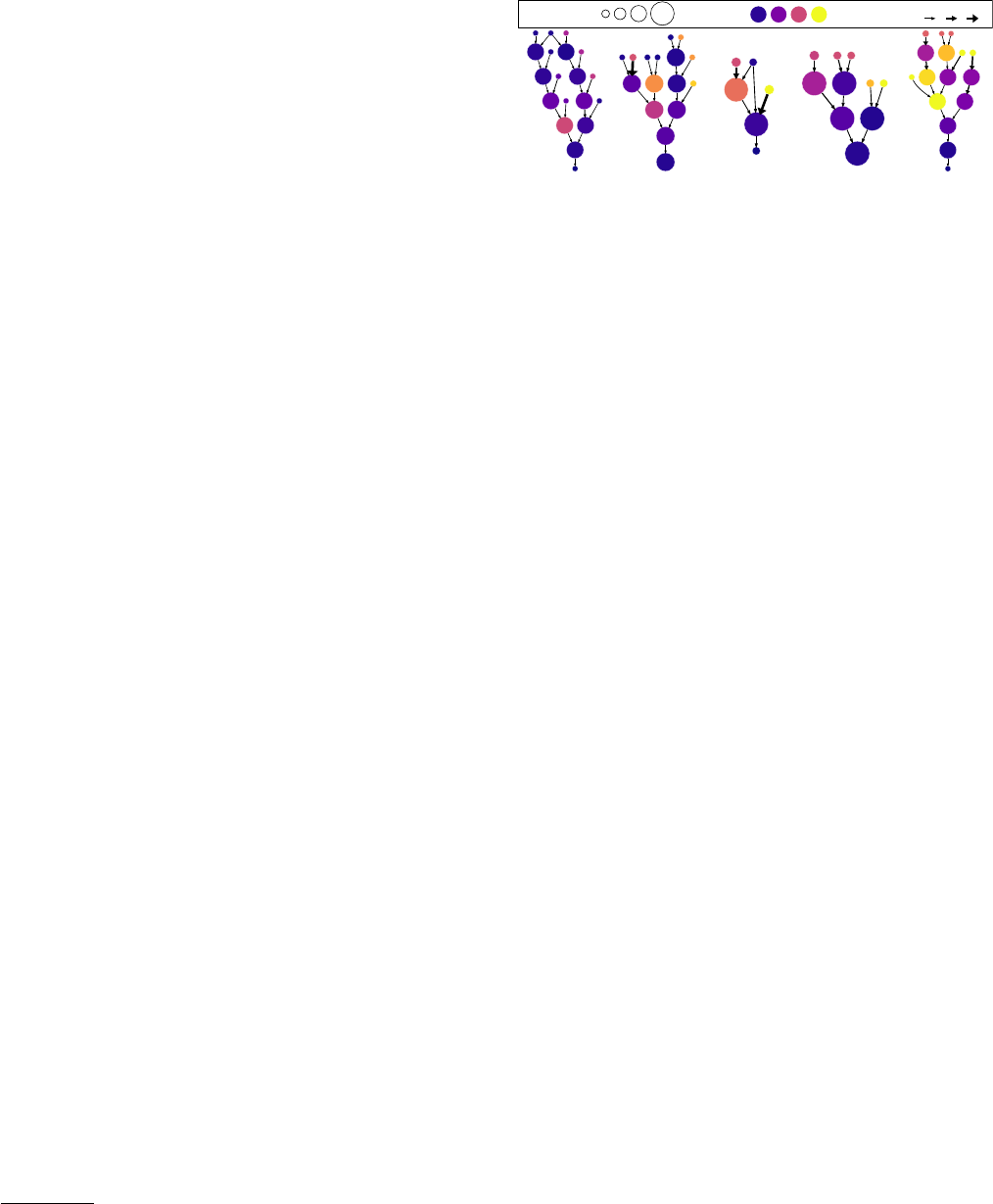
Figure 13:

Decima learns qualitatively different policies depending on the environment (e.g., costly (a) vs. free executor migration (b)) and the objective (e.g.,

average JCT (a) vs. makespan (c)). Vertical red lines indicate job completions, colors indicate tasks in different jobs, and dark purple is idle time.

     



























Figure 14:

Breakdown of each key idea’s contribution to Decima with

continuous job arrivals. Omitting any concept increases Decima’s average

JCT above that of the weighted fair policy.

Setup (IAT: interarrival time) Average JCT [sec]

Opt. weighted fair (best heuristic) 91.2±23.5

Decima, trained on test workload (IAT: 45 sec) 65.4±28.7

Decima, trained on anti-skewed workload (IAT: 75 sec) 104.8±37.6

Decima, trained on mixed workloads 82.3±31.2

Decima, trained on mixed workloads with interarrival time hints 76.6±33.4

Table 2:

Decima generalizes to changing workloads. For an unseen workload,

Decima outperforms the best heuristic by

10%

when trained with a mix of

workloads; and by 16% if it knows the interarrival time from an input feature.

inlong-horizon scheduling problems.Fourth,trainingonly on batched

job arrivals cannot generalize to continuous job arrivals. When trained

on batched arrivals, Decima learns to systematically defer large jobs,

as this results in the lowest sum of JCTs (lowest sum of penalties).

With continuous job arrivals, this policy starves large jobs indeﬁnitely

as the cluster load increases and jobs arrive more frequently. Conse-

quently, Decima underperforms the tuned weighted-fair heuristic at

loads above 65% when trained on batched arrivals.

Generalizing to different workloads.

We test Decima’s ability to

generalize by changing the training workload in the TPC-H experi-

ment (§7.2). To simulate shifts in cluster workload, we train models

for different job interarrival times between 42 and 75 seconds, and

test them using a workload with a 45 second interarrival time. As

Decima learns workload-speciﬁc policies, we expect its effectiveness

to depend on whether broad test workload characteristics, such as in-

terarrival time and job size distributions, match the training workload.

Table 2 shows the resulting average JCT. Decima performs well

when trained on a workload similar to the test workload. Unsur-

prisingly, when Decima trains with an “anti-skewed” workload (75

seconds interarrival time), it generalizes poorly and underperforms

the optimized weighted fair policy. This makes sense because Decima

incorporates the learned interarrival time distribution in its policy.

When training with a mixed set of workloads that cover the whole

interarrival time range, Decima can learn a more general policy. This

(a) Learning curve. (b) Scheduling delay.

Figure 15:

Different encodings of jobs parallelism (§5.2) affect Decima’s

training time. Decima makes low-latency scheduling decisions: on average,

the latency is about 50

smaller than the interval between scheduling events.

policy ﬁts less strongly to a speciﬁc interarrival time distribution and

therefore becomes more robust to workload changes. If Decima can

observe the interarrival time as a feature in its state (§6.1), it gener-

alizes better still and learns an adaptive policy that achieves a 16%

lower average JCT than the best heuristic. These results highlight that

a diverse training workload set helps make Decima’s learned policies

robust to workload shifts; we discuss possible online learning in §8.

Training and inference performance.

Figure 15a shows Decima’s

learning curve (in blue) on continuous TPC-H job arrivals (§7.2),

testing snapshots of the model every 100 iterations on (unseen) job

arrival sequences. Each training iteration takes about 5 seconds. Dec-

ima’s design (§5.3) is crucial for training efﬁciency: omitting the

parallelism limit values in the input (yellow curve) forces Decima to

use separate score functions for different limits, signiﬁcantly increas-

ing the number of parameters to optimize over; putting ﬁne-grained

parallelism control on nodes (green curve) slows down training as it

increases the space of algorithms Decima must explore.

Figure 15b shows cumulative distributions of the time Decima

takes to decide on a scheduling action (in red) and the time interval

between scheduling events (in blue) in our Spark testbed (§7.2). The

average scheduling delay for Decima is less than 15ms, while the

interval between scheduling events is typically in the scale of seconds.

In less than

of the cases, the scheduling interval is shorter than the

scheduling delay (e.g., when the cluster requests for multiple schedul-

ing actions in a single scheduling event). Thus Decima’s scheduling

delay imposes no measurable overhead on task runtimes.

8 Discussion

In this section, we discuss future research directions and other poten-

tial applications for Decima’s techniques.

SIGCOMM ’19, August 19-23, 2019, Beijing, China H. Mao et al.

Robustness and generalization.

Our experiments in §7.4 showed

that Decima can learn generalizable scheduling policies that work

well on anunseen workload. However, more drasticworkload changes

than interarrival time shifts could occur. To increase robustness of a

scheduling policy against such changes, it may be helpful to train the

agent on worst-case situations or adversarial workloads, drawing on

the emerging literature on robust adversarial RL [

]. Another direc-

tion is to adjust the scheduling policy online as the workload changes.

The key challenge with an online approach is to reduce the large sam-

ple complexity of model-free RL when the workload changes quickly.

One viable approach might be to use meta learning [

], which

allows training a “meta” scheduling agent that is designed to adapt

to a speciﬁc workload with only a few observations.

Other learning objectives.

In our experiments, we evaluated Dec-

ima on metrics related to job duration (e.g., average JCT, makespan).

Shaping the reward signal differently can steer Decima to meet other

objectives, too. For example, imposing a hard penalty whenever the

deadline of a job is missed would guide Decima to a deadline-aware

policy. Alternatively, basing the reward on e.g., the 90th percentile of

empirical job duration samples, Decima can optimize for a tight tail of

the JCT distribution. Addressing objectives formulated as constrained

optimization (e.g., to minimize average JCT, but strictly guarantee

fairness) using RL is an interesting further direction [2, 30].

Preemptive scheduling.

Decima currently never preempts running

tasks and can only remove executors from a job after a stage com-

pletes. This design choice keeps the MDP tractable for RL and results

in effective learning and strong scheduling policies. However, future

work might investigate more ﬁne-grained and reactive preemption

in an RL-driven scheduler such as Decima. Directly introducing pre-

emption would lead to a much larger action space (e.g., specifying

arbitrary set of executors to preempt) and might require a much higher

decision-making frequency. To make the RL problem tractable, one

potential research direction is to leverage multi-agent RL [

For example, a Decima-like scheduling agent might controls which

stage to run next and how many executors to assign, and, concurrently,

another agent might decide where to preempt executors.

Potential networking and system applications.

Some techniques

we developed for Decima are broadly applicable to other networking

and computer systems problems. For example, the scalable represen-

tation of input DAGs (§5.1) has applications in problems over graphs,

such as database query optimization [

] and hardware device place-

ment [

]. Our variance reduction technique (§5.3) generally applies

to systems with stochastic, unpredictable inputs [54, 55].

9 Related Work

There is little prior work on applying machine learning techniques

to cluster scheduling. DeepRM [

], which uses RL to train a neu-

ral network for multi-dimensional resource packing, is closest to

Decima in aim and approach. However, DeepRM only deals with

a basic setting in which each job is a single task and was evaluated

in simple, simulated environments. DeepRM’s learning model also

lacks support for DAG-structured jobs, and its training procedure

cannot handle realistic cluster workloads with continuous job arrivals.

In other applications, Mirhoseini et al.’s work on learning device

placement in TensorFlow (TF) computations [

] also uses RL, but

relies on recurrent neural networks to scan through all nodes for state

embedding, rather than a graph neural network. Their approach use re-

current neural networks to scan through all nodes for state embedding

instead of using a scalable graph neural network. The objective there

is to schedule a single TF job well, and the model cannot generalize

to unseen job combinations [59].

Prior work in machine learning and algorithm design has combined

RL and graph neural networks to optimize complex combinatorial

problems, such as vertex set cover and the traveling salesman prob-

lem [

]. The design of Decima’s scalable state representation is

inspired by this line of work, but we found that off-the-shelf graph

neural networks perform poorly for our problem. To train strong

scheduling agents, we had to change the graph neural network ar-

chitecture to enable Decima to compute, amongst other metrics, the

critical path of a DAG (§5.1).

For resource management systems more broadly, Paragon [

] and

Quasar [

] use collaborative ﬁltering to match workloads to different

machine types and avoid interference; their goal is complementary to

Decima’s. Tetrisched [

], like Decima, plans ahead in time, but uses

a constraint solver to optimize job placement and requires the user

to supply explicit constraints with their jobs. Firmament [

] also

uses a constraint solver and achieves high-quality placements, but

requires an administrator to conﬁgure an intricate scheduling policy.

Graphene [

] uses heuristics to schedule job DAGs, but cannot set

appropriate parallelism levels. Some systems “auto-scale” parallelism

levels to meet job deadlines [

] or opportunistically accelerate jobs

using spare resources [

, §5]. Carbyne [

] allows jobs to “altruisti-

cally” give up some of their short-term fair share of cluster resources

in order to improve JCT across jobs while guarantee long-term fair-

ness. Decima learns policies similar to Carbyne’s, balancing resource

shares and packing for low average JCT, but the current design of

Decima does not have fairness an objective.

General-purpose cluster managers like Borg [

], Mesos [

], or

YARN [

] support many different applications, making workload-

speciﬁcscheduling policies are difﬁcult toapply at this level. However,

Decima could run as a framework atop Mesos or Omega [68].

10 Conclusion

Decima demonstrates that automatically learning complex cluster

scheduling policies using reinforcement learning is feasible, and that

the learned policies are ﬂexible and efﬁcient. Decima’s learning inno-

vations, such as its graph embedding technique and the training frame-

work for streaming, may be applicable to other systems processing

DAGs(e.g., query optimizers). We will open source Decima, our mod-

els, and our experimental infrastructure at https://web.mit.edu/decima.

This work does not raise any ethical issues.

Acknowledgments.

We thank our shepherd, Aditya Akella, and the

SIGCOMM reviewers for their valuable feedback. We also thank

Akshay Narayan, Amy Ousterhout, Prateesh Goyal, Peter Iannucci,

and Songtao He for fruitful discussions throughout the development

of this project. We appreciate Haiyang Ding and Yihui Feng from

Alibaba Cloud Intelligence for sharing the production cluster dataset.

This work was funded in part by the NSF grants CNS-1751009,

CNS-1617702, a Google Faculty Research Award, an AWS Machine

Learning Research Award, a Cisco Research Center Award, an Alfred

P. Sloan Research Fellowship, and sponsors of the MIT DSAIL lab.

Learning Scheduling Algorithms for Data Processing Clusters SIGCOMM ’19, August 19-23, 2019, Beijing, China

References

[1]

Martín Abadi, Paul Barham, Jianmin Chen, Zhifeng Chen, Andy Davis, Jeffrey

Dean, Matthieu Devin, Sanjay Ghemawat, Geoffrey Irving, Michael Isard,

Manjunath Kudlur, Josh Levenberg, Rajat Monga, Sherry Moore, Derek G.

Murray, Benoit Steiner, Paul Tucker, Vijay Vasudevan, Pete Warden, Martin

Wicke, Yuan Yu, and Xiaoqiang Zheng. 2016. TensorFlow: A System for

Large-scale Machine Learning. In Proceedings of the 12

USENIX Confer-

ence on Operating Systems Design and Implementation (OSDI). 265–283.

http://dl.acm.org/citation.cfm?id=3026877.3026899

[2]

Joshua Achiam, David Held, Aviv Tamar, and Pieter Abbeel. 2017. Constrained

policy optimization. In Proceedings of the 34

International Conference on

Machine Learning-Volume 70. 22–31.

[3]

Ravichandra Addanki, Shaileshh Bojja Venkatakrishnan, Shreyan Gupta, Hongzi

Mao, and Mohammad Alizadeh. 2018. Placeto: Efﬁcient Progressive Device

Placement Optimization. In Proceedings of the 1

Machine Learning for Systems

Workshop.

[4]

Sameer Agarwal, Srikanth Kandula, Nicolas Bruno, Ming-Chuan Wu, Ion Stoica,

and Jingren Zhou. 2012. Re-optimizing Data-parallel Computing. In Proceedings

of the 9

USENIX Conference on Networked Systems Design and Implementation

(NSDI). 281–294. http://dl.acm.org/citation.cfm?id=2228298.2228327

[5]

Kunal Agrawal, Jing Li, Kefu Lu, and Benjamin Moseley. 2016. Scheduling

parallel DAG jobs online to minimize average ﬂow time. In Proceedings of the

annual ACM-SIAM symposium on Discrete Algorithms (SODA). Society for

Industrial and Applied Mathematics, 176–189.

[6]

Alibaba. 2017. Cluster data collected from production clusters in Alibaba for

cluster management research. https://github.com/alibaba/clusterdata. (2017).

[7]

Dario Amodei and Danny Hernandez. 2018. AI and Compute.

https://openai.com/blog/ai-and-compute/. (2018).

[8]

Apache Hadoop. 2014. Hadoop Fair Scheduler. (2014). http:

//hadoop.apache.org/common/docs/stable1/fair_scheduler.html

[9]

Apache Spark. 2018. Spark: Dynamic Resource Allocation. (2018). http:

//spark.apache.org/docs/2.2.1/job-scheduling.html#dynamic-resource-allocation

Spark v2.2.1 Documentation.

[10] Apache Tez 2013. Apache Tez Project. https://tez.apache.org/. (2013).

[11]

Luiz André Barroso, Jimmy Clidaras, and Urs Hölzle. 2013. The Datacenter

as a Computer: An Introduction to the Design of Warehouse-Scale Machines,

second edition. Synthesis Lectures on Computer Architecture 8, 3 (July 2013).

https://doi.org/10.2200/S00516ED2V01Y201306CAC024

[12]

Peter W. Battaglia, Jessica B. Hamrick, Victor Bapst, Alvaro Sanchez-Gonzalez,

Vinícius Flores Zambaldi, Mateusz Malinowski, Andrea Tacchetti, David Raposo,

Adam Santoro, Ryan Faulkner, Çaglar Gülçehre, Francis Song, Andrew J.

Ballard, Justin Gilmer, George E. Dahl, Ashish Vaswani, Kelsey Allen, Charles

Nash, Victoria Langston, Chris Dyer, Nicolas Heess, Daan Wierstra, Pushmeet

Kohli, Matthew Botvinick, Oriol Vinyals, Yujia Li, and Razvan Pascanu. 2018.

Relational inductive biases, deep learning, and graph networks. arXiv preprint

arXiv:1806.01261 (2018).

[13]

Richard Bellman. 1966. Dynamic programming. Science 153, 3731 (1966), 34–37.

[14]

Yoshua Bengio, Jérôme Louradour, Ronan Collobert, and Jason Weston. 2009.

Curriculum learning. In Proceedings of the 26

annual International Conference

on Machine Learning (ICML). 41–48.

[15]

Dimitri P Bertsekas and John N Tsitsiklis. 1995. Neuro-dynamic programming:

an overview. In Decision and Control, 1995., Proceedings of the 34th IEEE

Conference on, Vol. 1. IEEE, 560–564.

[16]

Arka A. Bhattacharya, David Culler, Eric Friedman, Ali Ghodsi, Scott Shenker,

and Ion Stoica. 2013. Hierarchical Scheduling for Diverse Datacenter Workloads.

In Proceedings of the 4

Annual Symposium on Cloud Computing (SoCC). Article

4, 15 pages. https://doi.org/10.1145/2523616.2523637

[17]

Christopher M. Bishop. 2006. Pattern Recognition and Machine Learning.

Springer.

[18]

Robert D Blumofe and Charles E Leiserson. 1999. Scheduling multithreaded

computations by work stealing. Journal of the ACM (JACM) 46, 5 (1999), 720–748.

[19]

Craig Chambers, Ashish Raniwala, Frances Perry, Stephen Adams, Robert R.

Henry, Robert Bradshaw, and Nathan Weizenbaum. 2010. FlumeJava: Easy,

Efﬁcient Data-parallel Pipelines. In Proceedings of the 2010 ACM SIGPLAN

Conference on Programming Language Design and Implementation (PLDI).

363–375. https://doi.org/10.1145/1806596.1806638

[20]

Chandra Chekuri, Ashish Goel, Sanjeev Khanna, and Amit Kumar. 2004. Multi-

processor scheduling to minimize ﬂow time with

resource augmentation. In Pro-

ceedings of the 36

Annual ACM Symposium on Theory of Computing. 363–372.

[21]

Dilip Chhajed and Timothy J Lowe. 2008. Building intuition: insights from basic

operations management models and principles. Vol. 115. Springer Science &

Business Media.

[22]

Ignasi Clavera, Jonas Rothfuss, John Schulman, Yasuhiro Fujita, Tamim Asfour,

and Pieter Abbeel. 2018. Model-based reinforcement learning via meta-policy

optimization. arXiv preprint arXiv:1809.05214 (2018).

[23]

Hanjun Dai, Elias B. Khalil, Yuyu Zhang, Bistra Dilkina, andLe Song. 2017. Learn-

ing Combinatorial Optimization Algorithms overGraphs. In Proceedings of the 31

Conference on Neural Information Processing Systems (NeurIPS). 6348–6358.

[24]

Michaël Defferrard, Xavier Bresson, and Pierre Vandergheynst. 2016. Convolu-

tional Neural Networks on Graphs with Fast Localized Spectral Filtering. arXiv

preprint arXiv:1606.09375 (2016).

[25]

Christina Delimitrou and Christos Kozyrakis. 2013. Paragon: QoS-aware Sched-

uling for Heterogeneous Datacenters. In Proceedings of the 18

International

Conference on Architectural Support for Programming Languages and Operating

Systems (ASPLOS). 77–88. https://doi.org/10.1145/2451116.2451125

[26]

Christina Delimitrou and Christos Kozyrakis. 2014. Quasar: Resource-efﬁcient

and QoS-aware Cluster Management. In Proceedings of the 19

International

Conference on Architectural Support for Programming Languages and Operating

Systems (ASPLOS). 127–144. https://doi.org/10.1145/2541940.2541941

[27]

Yan Duan, John Schulman, Xi Chen, Peter L Bartlett, Ilya Sutskever, and Pieter

Abbeel. 2016. RL2: Fast Reinforcement Learning via Slow Reinforcement

Learning. arXiv preprint arXiv:1611.02779 (2016).

[28]

Andrew D Ferguson, Peter Bodik, Srikanth Kandula, Eric Boutin, and Rodrigo Fon-

seca. 2012. Jockey: guaranteed job latency in data parallel clusters. In Proceedings

of the 7

ACM European Conference on Computer Systems (EuroSys).

[29]

Chelsea Finn, Pieter Abbeel, and Sergey Levine. 2017. Model-Agnostic

Meta-Learning for Fast Adaptation of Deep Networks. In Proceedings of the 34

International Conference on Machine Learning (ICML). 1126–1135.

[30]

Peter Geibel. 2006. Reinforcement learning for MDPs with constraints. In Proceed-

ings of the 17

European Conference on Machine Learning (ECML). 646–653.

[31]

Ali Ghodsi, Matei Zaharia, Benjamin Hindman, Andy Konwinski, Scott

Shenker, and Ion Stoica. 2011. Dominant Resource Fairness: Fair Allocation

of Multiple Resource Types. In Proceedings of the 8

USENIX Sympo-

sium on Networked Systems Design and Implementation (NSDI). 323–336.

http://dl.acm.org/citation.cfm?id=1972457.1972490

[32]

Ali Ghodsi, Matei Zaharia, Scott Shenker, and Ion Stoica. 2013. Choosy:

max-min fair sharing for datacenter jobs with constraints. In Proceedings of

the 8

ACM European Conference on Computer Systems (EuroSys). 365–378.

https://doi.org/10.1145/2465351.2465387

[33]

Ionel Gog, Malte Schwarzkopf, Adam Gleave, Robert N. M. Watson, and

Steven Hand. 2016. Firmament: fast, centralized cluster scheduling at scale. In

Proceedings of the 12

USENIX Symposium on Operating Systems Design and

Implementation (OSDI). 99–115.

[34]

Robert Grandl, Ganesh Ananthanarayanan, Srikanth Kandula, Sriram Rao,

and Aditya Akella. 2014. Multi-resource Packing for Cluster Schedulers. In

Proceedings of the 2014 ACM SIGCOMM Conference (SIGCOMM). 455–466.

[35]

Robert Grandl, Mosharaf Chowdhury, Aditya Akella, and Ganesh Anantha-

narayanan. 2016. Altruistic Scheduling in Multi-resource Clusters. In Proceedings

of the 12

USENIX Conference on Operating Systems Design and Implementation

(OSDI). 65–80. http://dl.acm.org/citation.cfm?id=3026877.3026884

[36]

Robert Grandl, Srikanth Kandula, Sriram Rao, Aditya Akella, and Janardhan

Kulkarni. 2016. Graphene: Packing and dependency-aware scheduling for

data-parallel clusters. In Proceedings of the 12

USENIX Symposium on Operating

Systems Design and Implementation (OSDI). 81–97.

[37]

Evan Greensmith, Peter L Bartlett, and Jonathan Baxter. 2004. Variance reduction

techniques for gradient estimates in reinforcement learning. Journal of Machine

Learning Research 5, Nov (2004), 1471–1530.

[38]

Jayesh K Gupta, Maxim Egorov, and Mykel Kochenderfer. 2017. Cooperative

multi-agent control using deep reinforcement learning. In Proceedings of the

2017 International Conference on Autonomous Agents and Multiagent Systems

(AAMAS). 66–83.

[39]

Martin T Hagan, Howard B Demuth, Mark H Beale, and Orlando De Jesús. 1996.

Neural network design. PWS publishing company Boston.

[40]

W Keith Hastings. 1970. Monte Carlo sampling methods using Markov chains

and their applications. Biometrika 1 (1970).

[41]

Benjamin Hindman, Andy Konwinski, Matei Zaharia, Ali Ghodsi, Anthony D

Joseph, Randy H Katz, Scott Shenker, and Ion Stoica. 2011. Mesos: A Platform

for Fine-Grained Resource Sharing in the Data Center. In Proceedings of the 8

USENIX Conference on Networked Systems Design and Implementation (NSDI).

[42]

Michael Isard, Mihai Budiu, Yuan Yu, Andrew Birrell, and Dennis Fetterly. 2007.

Dryad: Distributed Data-parallel Programs from Sequential Building Blocks. In

Proceedings of the 2

ACM SIGOPS/EuroSys European Conference on Computer

Systems (EuroSys). 59–72. https://doi.org/10.1145/1272996.1273005

[43]

Michael Isard, Vijayan Prabhakaran, Jon Currey, Udi Wieder, Kunal Talwar, and

Andrew Goldberg. 2009. Quincy: fair scheduling for distributed computing clusters.

In Proceedings of the 22

ACM Symposium on Operating Systems Principles

(SOSP). 261–276. https://doi.org/10.1145/1629575.1629601

[44]

James E. Kelley Jr and Morgan R. Walker. 1959. Critical-path planning and

scheduling. In Proceedings of the Eastern Joint IRE-AIEE-ACM Computer

Conference (EJCC). 160–173.

SIGCOMM ’19, August 19-23, 2019, Beijing, China H. Mao et al.

[45]

Diederik P Kingma and Jimmy Ba. 2015. Adam: A method for stochastic

optimization. Proceedings of the 7

International Conference on Learning

Representations (ICLR) (2015).

[46]

Thomas N. Kipf and Max Welling. 2016. Semi-Supervised Classiﬁcation with

Graph Convolutional Networks. arXiv preprint arXiv:1609.02907 (2016).

http://arxiv.org/abs/1609.02907

[47]

Prasad A. Kulkarni. 2011. JIT compilation policy for modern machines. In ACM

SIGPLAN Notices, Vol. 46. 773–788.

[48]

Tom Leighton, Bruce Maggs, and Satish Rao. 1988. Universal packet routing

algorithms. In Proceedings of the 29

annual Symposium on Foundations of

Computer Science (FOCS). 256–269.

[49]

Zhuwen Li, Qifeng Chen, and Vladlen Koltun. 2018. Combinatorial optimization

with graph convolutional networks and guided tree search. In Proceedings of the

Conference on Neural Information Processing Systems (NeurIPS). 539–548.

[50]

Eric Liang and Richard Liaw. 2018. Scaling Multi-Agent Reinforcement Learning.

https://bair.berkeley.edu/blog/2018/12/12/rllib/. (2018).

[51]

Timothy P Lillicrap, Jonathan J Hunt, Alexander Pritzel, Nicolas Heess, Tom Erez,

Yuval Tassa, David Silver, and Daan Wierstra. 2015. Continuous control with deep

reinforcement learning. arXiv preprint arXiv:1509.02971 (2015).

[52]

Chengzhi Lu, Kejiang Ye, Guoyao Xu, Cheng-Zhong Xu, and Tongxin Bai. 2017.

Imbalance in the cloud: An analysis on alibaba cluster trace. In Proceedings of the

2017 IEEE International Conference on Big Data (BigData). IEEE, 2884–2892.

[53]

Hongzi Mao, Mohammad Alizadeh, Ishai Menache, and Srikanth Kandula. 2016.

Resource Management with Deep Reinforcement Learning. In Proceedings of the

ACM Workshop on Hot Topics in Networks (HotNets).

[54]

Hongzi Mao, Shannon Chen, Drew Dimmery, Shaun Singh, Drew Blaisdell,

Yuandong Tian, Mohammad Alizadeh, and Eytan Bakshy. 2019. Real-world

Video Adaptation with Reinforcement Learning. In Proceedings of the 2019

Reinforcement Learning for Real Life Workshop.

[55]

Hongzi Mao, Shaileshh Bojja Venkatakrishnan, Malte Schwarzkopf, and

Mohammad Alizadeh. 2019. Variance Reduction for Reinforcement Learning in

Input-Driven Environments. Proceedings of the 7

International Conference on

Learning Representations (ICLR) (2019).

[56]

Ryan Marcus, Parimarjan Negi, Hongzi Mao, Chi Zhang, Mohammad Alizadeh,

Tim Kraska, Olga Papaemmanouil, and Nesime Tatbul. 2019. Neo: A Learned

Query Optimizer. arXiv preprint arXiv:1904.03711 (2019).

[57]

Monaldo Mastrolilli and Ola Svensson. 2008. (Acyclic) job shops are hard to

approximate. In Proceedings of the 49

IEEE Symposium on Foundations of

Computer Science (FOCS). 583–592.

[58]

Ishai Menache, Shie Mannor, and Nahum Shimkin. 2005. Basis functionadaptation

in temporal difference reinforcement learning. Annals of Operations Research

134, 1 (2005), 215–238.

[59]

Azalia Mirhoseini, Anna Goldie, Hieu Pham, Benoit Steiner, Quoc V Le, and Jeff

Dean. 2018. A Hierarchical Model for Device Placement. In Proceedings of the

International Conference on Learning Representations (ICLR).

[60]

Azalia Mirhoseini, Hieu Pham, Quoc V Le, Benoit Steiner, Rasmus Larsen,

Yuefeng Zhou, Naveen Kumar, Mohammad Norouzi, Samy Bengio, and Jeff

Dean. 2017. Device Placement Optimization with Reinforcement Learning. In

Proceedings of the 33

International Conference on Machine Learning (ICML).

[61]

Volodymyr Mnih, Koray Kavukcuoglu, David Silver, Andrei A. Rusu, Joel Veness,

Marc G. Bellemare, Alex Graves, Martin Riedmiller, Andreas K. Fidjeland, Georg

Ostrovski, Stig Petersen, Charles Beattie, Amir Sadik, Ioannis Antonoglou, Helen

King, Dharshan Kumaran, Daan Wierstra, Shane Legg, Demis Hassabis, Ioannis

Antonoglou, Daan Wierstra, and Martin A. Riedmiller. 2015. Human-level control

through deep reinforcement learning. Nature 518 (2015), 529–533.

[62]

Thanh Thi Nguyen, Ngoc Duy Nguyen, and Saeid Nahavandi. 2018. Deep

Reinforcement Learning for Multi-Agent Systems: A Review of Challenges,

Solutions and Applications. arXiv preprint arXiv:1812.11794 (2018).

[63]

Kay Ousterhout, Ryan Rasti, Sylvia Ratnasamy, Scott Shenker, and

Byung-Gon Chun. 2015. Making Sense of Performance in Data Ana-

lytics Frameworks. In Proceedings of the 12

USENIX Symposium on

Networked Systems Design and Implementation (NSDI). 293–307. https:

//www.usenix.org/conference/nsdi15/technical-sessions/presentation/ousterhout

[64]

Lerrel Pinto, James Davidson, Rahul Sukthankar, and Abhinav Gupta. 2017. Robust

Adversarial Reinforcement Learning. In Proceedings of the 34

International

Conference on Machine Learning (ICML). 2817–2826.

[65]

Chandrasekharan Rajendran. 1994. A no-wait ﬂowshop scheduling heuristic to

minimize makespan. Journal of the Operational Research Society 45, 4 (1994),

472–478.

[66]

Jeff Rasley, Konstantinos Karanasos, Srikanth Kandula, Rodrigo Fonseca, Milan

Vojnovic, and Sriram Rao. 2016. Efﬁcient Queue Management for Cluster

Scheduling. In Proceedings of the 11

European Conference on Computer Systems

(EuroSys). Article 36, 15 pages. https://doi.org/10.1145/2901318.2901354

[67]

John Schulman, Sergey Levine, Pieter Abbeel, Michael Jordan, and Philipp Moritz.

2015. Trust region policy optimization. In Proceedings of the 32nd International

Conference on Machine Learning (ICML). 1889–1897.

[68]

Malte Schwarzkopf, Andy Konwinski, Michael Abd-El-Malek, and John Wilkes.

2013. Omega: ﬂexible, scalable schedulers for large compute clusters. In

Proceedings of the 8

ACM European Conference on Computer Systems (EuroSys).

351–364.

[69]

David B Shmoys, Clifford Stein, and Joel Wein. 1994. Improved approximation

algorithms for shop scheduling problems. SIAM J. Comput. 23, 3 (1994), 617–632.

[70]

David Silver, Aja Huang, Christopher J. Maddison, Arthur Guez, Laurent Sifre,

George van den Driessche, Julian Schrittwieser, Ioannis Antonoglou, Veda

Panneershelvam, Marc Lanctot, Sander Dieleman, Dominik Grewe, John Nham,

Nal Kalchbrenner, Ilya Sutskever, Timothy Lillicrap, Madeleine Leach, Koray

Kavukcuoglu, Thore Graepel, and Demis Hassabis. 2016. Mastering the game

of Go with deep neural networks and tree search. Nature 529 (2016), 484–503.

[71]

David Silver, Julian Schrittwieser, Karen Simonyan, Ioannis Antonoglou, Aja

Huang, Arthur Guez, Thomas Hubert, Lucas Baker, Matthew Lai, Adrian Bolton,

Yutian Chen, Timothy Lillicrap, Fan Hui, Laurent Sifre, George van den Driessche,

Thore Graepel, and Demis Hassabis. 2017. Mastering the game of Go without

human knowledge. Nature 550, 7676 (2017), 354.

[72]

Richard. S. Sutton and Andrew. G. Barto. 2017. Reinforcement Learning: An

Introduction, Second Edition. MIT Press.

[73] TPC-H 2018. The TPC-H Benchmarks. www.tpc.org/tpch/. (2018).

[74]

Alexey Tumanov, Timothy Zhu, Jun Woo Park, Michael A. Kozuch, Mor

Harchol-Balter, and Gregory R. Ganger. 2016. TetriSched: Global Rescheduling

with Adaptive Plan-ahead in Dynamic Heterogeneous Clusters. In Proceedings

of the 11

European Conference on Computer Systems (EuroSys). Article 35,

16 pages. https://doi.org/10.1145/2901318.2901355

[75]

Vinod Kumar Vavilapalli, Arun C. Murthy, Chris Douglas, Sharad Agarwal, Ma-

hadev Konar, Robert Evans, Thomas Graves, Jason Lowe, Hitesh Shah, Siddharth

Seth, Bikas Saha, Carlo Curino, Owen O’Malley, Sanjay Radia, Benjamin Reed,

and Eric Baldeschwieler. 2013. Apache Hadoop YARN: Yet Another Resource

Negotiator. In Proceedings of the 4

annual Symposium on Cloud Computing

(SoCC). Article 5, 16 pages. https://doi.org/10.1145/2523616.2523633

[76]

Abhishek Verma, Madhukar Korupolu, and John Wilkes. 2014. Evaluating

job packing in warehouse-scale computing. In Proceedings of the 2014 IEEE

International Conference on Cluster Computing (CLUSTER). 48–56.

[77]

Abhishek Verma, Luis Pedrosa, Madhukar R. Korupolu, David Oppenheimer,

Eric Tune, and John Wilkes. 2015. Large-scale cluster management at Google

with Borg. In Proceedings of the 10

European Conference on Computer Systems

(EuroSys). Bordeaux, France.

[78]

Lex Weaver and Nigel Tao. 2001. The optimal reward baseline for gradient-based

reinforcement learning. In Proceedings of the 17

Conference on Uncertainty in

Artiﬁcial Intelligence (UAI). 538–545.

[79]

Ronald J Williams. 1992. Simple statistical gradient-following algorithms for

connectionist reinforcement learning. Machine learning 8, 3-4 (1992), 229–256.

[80]

Matei Zaharia, Mosharaf Chowdhury, Tathagata Das, Ankur Dave, Justin

Ma, Murphy McCauley, Michael J. Franklin, Scott Shenker, and Ion Sto-

ica. 2012. Resilient Distributed Datasets: A Fault-tolerant Abstraction for

In-memory Cluster Computing. In Proceedings of the 9

USENIX Con-

ference on Networked Systems Design and Implementation (NSDI). 15–28.

http://dl.acm.org/citation.cfm?id=2228298.2228301

Learning Scheduling Algorithms for Data Processing Clusters SIGCOMM ’19, August 19-23, 2019, Beijing, China

Appendices

Appendices are supporting material that has not been peer reviewed.

A An example of dependency-aware scheduling

Critical path: 28 + 3ϵ

(# tasks, task duration)

(5, ϵ)

(1, 10)

(40, 1)

(5, ϵ)

(5, 10)

(5, ϵ)

Optimal: 20 + 3ϵ

8 ϵ

2ϵ 10

Time

Task slots

Time

Task slots

2ϵ 10

Figure 16:

An optimal DAG-aware schedule plans ahead and parallelizes

execution of the blue and green stages, so that orange and green stages

complete at the same time and the bottom join stage can execute immediately.

A straightforward critical path heuristic would instead focus on the right

branch, and takes 29% longer to execute the job.

Directed acyclic graphs (DAGs) of dependent operators or “stages”

are common in parallel data processing applications. Figure 16 shows

a common example: a DAG with two branches that converge in a join

stage. A simple critical path heuristic would choose to work on the

right branch, whichcontains more aggregatework: 90task-seconds vs.

10 task-seconds in the left branch. With this choice, once the orange

stage ﬁnishes, however, the ﬁnal join stage cannot run, since its other

parent stage (in green) is still incomplete. Completing the green stage

next, followed by the join stage — as a critical-path schedule would —

results in an overall makespan of

28+ 3ϵ

. The optimal schedule, by

contrast, completes this DAG in

20+3ϵ

time, 29% faster. Intuitively,

an ideal schedule allocates resources such that both branches reach

the ﬁnal join stage at the same time, and execute it without blocking.

B Background on Reinforcement Learning

We brieﬂy review reinforcement learning (RL) techniques that we use

in this paper; for a detailed survey and rigorous derivations, see e.g.,

Sutton and Barto’s book [72].

Reinforcement learning.

Consider the general setting in Figure 17,

where an RL agent interacts with an environment. At each step

, the

agent observes some state

, and takes an action

. Following the

action, the state of the environment transitions to

k+1

and the agent

receives a reward

as feedback. The state transitions and rewards are

stochastic and assumed to be a Markov process: the state transition

k+1

and the reward

depend only on the state

and the action

at step k (i.e., they are conditionally independent of the past).

In the general RL setting, the agent only controls its actions: it

has no a priori knowledge of the state transition probabilities or the

reward function. However, by interacting with the environment, the

agent can learn these quantities during training.

For training, RL proceeds in episodes. Each episode consists of

a sequence of (state, action, reward) observations— i.e.,

)

at each step

k ∈ [0,1,. . .,T ]

, where

is the episode length . For ease of

understanding, we ﬁrst describe an RL formulation that maximizes

Agent

State

Neural

network

Policy

, a

)

Environment

Take action a

Observe state s

Reward r

Parameter θ

Figure 17:

A reinforcement learning setting with neural networks [

The policy is parameterized using a neural network and is trained iteratively

via interactions with the environment that observe its state and take actions.

the total reward:

k=0

. However, in our scheduling problem,

the average reward formulation (§5.3) is more suitable. We later de-

scribe how to modify the reward signal to convert the objective to the

average reward setting.

Policy.

The agent picks actions based on a policy

π(s

)

, deﬁned

as a probability of taking action

at state

. In most practical

problems, the number of possible

{

state, action

}

pairs is too large

to store the policy in a lookup table. It is therefore common to use

function approximators [

], with a manageable number of ad-

justable parameters,

, to represent the policy as

, a

)

. Many

forms of function approximators can be used to represent the pol-

icy. Popular choices include linear combinations of features of the

state/action space (i.e.,

)= θ

ϕ(s

)

), and, recently, neural

networks [

] for solve large-scale RL tasks [

]. An advantage

of neural networks is that they do not need hand-crafted features, and

that they are end-to-end differentiable for training.

Policy gradient methods.

We focus on a class of RL algorithms that

perform training by using gradient-descent on the policy parameters.

Recall that the objective is to maximize the expected total reward; the

gradient of this objective is given by:

∇

k=0

= E

k=0

∇

logπ

)

, (4)

where

)

is the expected total discounted reward from (de-

terministically) choosing action

in state

, and subsequently fol-

lowing policy

[

, §13.2]. The key idea in policy gradient methods

is to estimate the gradient using the trajectories of execution with the

current policy. Following the Monte Carlo Method [

], the agent

samples multiple trajectories and uses the empirical total discounted

reward,

, as an unbiased estimate of

)

. It then updates

the policy parameters via gradient descent:

θ ←θ + α

k=0

∇

logπ

, (5)

where

is the learning rate. This equation results in the REINFORCE

algorithm [

]. The intuition of REINFORCE is that the direction

∇

logπ

, a

)

indicates how to change the policy parameters in

order to increase

)

(the probability of action

at state

Equation 5 takes a step in this direction; the size of the step depends

on the magnitude of the return

. The net effect is to reinforce actions

SIGCOMM ’19, August 19-23, 2019, Beijing, China H. Mao et al.

that empirically lead to better returns. Appendix C describes how we

implement this training method in practice.

Policy gradient methods are better suited to our scheduling context

than the alternative value-basedmethods for tworeasons. First, policy-

based methods are easier to design if it is unclear whether the neural

network architecture used has adequate expressive power. The reason

is that value-based methods aim to ﬁnd a ﬁxed-point of the Bellman

equations [

]. If the underlying neural network cannot express the

optimal value function, then a value-based method can have difﬁculty

converging because the algorithm is trying to converge to a ﬁxedpoint

that the neural network cannot express. With policy-based methods,

this issue does not arise, because regardless of the policy network’s

expressive power, the policy gradient algorithm will optimize for the

reward objective over the space of policies that the neural network

can express. Second, policy gradient methods allow us to use input-

dependent baselines [

] to reduce training variance (challenge #2 in

§5.3). It is currently unknown whether, and how, this technique can

be applied to value-based methods.

Average reward formulation.

For our scheduling problem, an aver-

age reward formulation, which maximizes

lim

T →∞

1/T

k=0

is a better objective than the total reward we discussed so far.

To convert the objective from the sum of rewards to the average

reward, we replace the reward

with a differential reward. Opera-

tionally, at every step

, the environment modiﬁes the reward to the

agent as

←r

−

, where

is a moving average of the rewards across

alargenumberof previoussteps(across manytraining episodes). With

this modiﬁcation, we can reuse the same policy gradient method as in

Equation

(4)

and

(5)

to ﬁnd the optimal policy. Sutton and Barto [

§10.3, §13.6] describe the mathematical details on how this approach

optimizes the average reward objective.

C Training implementation details

Algorithm 1 presents the pseudocode for Decima’s training procedure

as described in §5.3. In particular, line 3 samples the episode length

from an exponential distribution, with a small initial mean

mean

. This

step terminates the initial episodes early to avoid wasting training

time (see challenge #1 in §5.3). Then, we sample a job sequence (line

4) and use it to collect

episodes of experience (line 5). Importantly,

the baseline

in line 8 is computed with the same job sequence

to reduce the variance caused by the randomness in the job arrival

process (see challenge #2in §5.3). Line10 is the policygradient REIN-

FORCE algorithm described in Eq.

(3)

. Line 13 increases the average

episode length (i.e., the curriculum learning procedure for challenge

#1 in §5.3). Finally, we update Decima’s policy parameter

on line 14.

Our neural network architecture is described in §6.1, and we set

the hyperparameters in Decima’s training as follows. The number of

incoming jobs is capped at 2000, and the episode termination prob-

ability decays linearly from

5×10

−7

5×10

−8

throughout training.

The learning rate

1×10

−3

and we use Adam optimizer [

] for

gradient descent. For continuous job arrivals, the moving window for

estimating

spans

time steps (see the average reward formulation

in Appendix B). Finally, we train Decima for at least 50,000 iterations

for all experiments.

Weimplemented Decima’s training frameworkusing TensorFlow[

and we use 16 workers to compute episodes with the same job se-

quence in parallel during training. Each training iteration, including

Algorithm 1 Policy gradient method used to train Decima.

1: for each iteration do

2: ∆θ ← 0

3: Sample episode length τ ∼ exponential(τ

mean

)

4: Sample a job arrival sequence

5: Run episodes i = 1,. . .,N :

,. . .,s

} ∼π

6: Compute total reward: R

′

7: for k = 1 to τ do

8: compute baseline: b

i=1

9: for i = 1 to N do

10: ∆θ ← ∆θ + ∇

logπ

)(R

−b

)

11: end for

12: end for

13: τ

mean

←τ

mean

+ϵ

14: θ ←θ +α∆θ

15: end for

interaction with the simulator, model inference and model update

from all training workers, takes roughly 1.5 seconds on a machine

with Intel Xeon E5-2640 CPU and Nvidia Tesla P100 GPU.

All experiments in §7 are performed on test job sequences unseen

during training (e.g., unseen TPC-H job combinations, unseen part

of the Alibaba production trace, etc.).

D Simulator ﬁdelity

Our training infrastructure relies on a faithful simulator of Spark job

execution in a cluster.Tovalidatethe simulator’s ﬁdelity, we measured

how simulated and real Spark differ in terms of job completion time

for ten runs of TPC-H job sets (§7.2), both when jobs run alone and

when they share a cluster with other jobs. Figure 18 shows the results:

the simulator closely matches the actual run time of each job, even

when we run multiple jobs together in the cluster. In particular, the

mean error of our simulation is within

of real runtime when jobs

run in isolation, and within

when sharing a cluster (95

percentile:

≤ 10% in isolation, ≤ 20% when sharing).

We found that capturing all ﬁrst-order effects of the Spark envi-

ronment is crucial to achieving this accuracy (§6.2). For example,

without modeling the delay to move an executor between jobs, the

simulated runtime consistently underapproximates reality. Training

in such an environment would result in a policy that moves executors

more eagerly than is actually sensible (§7.4). Likewise, omitting the

effects of initial and subsequent “waves” of tasks, or the slowdown

overheads imposed with high degrees of paralllism, signiﬁcantly in-

creases the variance in simulated runtime and makes it more difﬁcult

for Decima to learn a good policy.

E Expressiveness of Decima’s state representation

Decima’s can only learn strong scheduling policies if its state repre-

sentation, embedding scheme, and neural network architecture can

express them (§7).

In Equation

(1)

, combining two non-linear transforms

f (·)

and

д(·)

enablesDecima to express a wide variety ofaggregationfunctions. For

example, if

f ∼ log(·/n)

д ∼ exp(n×·)

, and

n → ∞

, the aggregation

computes the maximum of the child node embeddings. By contrast,

a standard aggregation operation of the form

u ∈ξ (v)

f (e

)

Learning Scheduling Algorithms for Data Processing Clusters SIGCOMM ’19, August 19-23, 2019, Beijing, China

(a) Single job running in isolation.

(b) Mixture of jobs on a shared cluster.

Figure 18:

Testing the ﬁdelity of our Spark simulator with Decima as a

scheduling agent. Blue bars in the upper part show the absolute real Spark job

duration (error bars: standard deviation across ten experiments); the orange

bars in the lower ﬁgures show the distribution of simulation error for a

95%

conﬁdence interval. The mean discrepancy between simulated and actual job

duration is at most ±5% for isolated, single jobs, and the mean error for a mix

of all 22 queries running on the cluster is at most ±9%.

0 50 100 150 200 250 300 350

Number of iterations

40%

60%

80%

100%

Testing accuracy

Single non-linear aggregation

Decima's two-level aggregation

Figure 19:

Trained using supervised learning, Decima’s two-level non-linear

transformation is able to express the max operation necessary for computing

the critical path (§5.1), and consequently achieves near-perfect accuracy on

unseen DAGs compared to the standard graph embedding scheme.

without a second non-linear transformation

д(·)

is insufﬁcient to

express the max operation. Consequently, such an architecture cannot

learn the aggregation (max) required to ﬁnd the critical path of a graph.

During development, we relied on a simple sanity check to test

the expressiveness of a graph embedding scheme. We used super-

vised learning to train the graph neural network to output the critical

path value of each node in a large number of random graphs, and

then checked how accurately the graph neural network identiﬁed

the node with the maximum critical path value. Figure 19 shows the

testing accuracy that Decima’s node embedding with two aggregation

levels achieves on unseen graphs, and compares it to the accuracy

achieved by a simple, single-level embedding with only one non-

linear transformation. Decima’s node embedding manages to learn

the max operation and therefore accurately identiﬁes the critical path

after about 150 iterations, while the standard embedding is incapable

of expressing the critical path and consequently never reaches a stable

high accuracy.

F Multi-resource scheduling heuristic comparison details

When evaluating Decima’s performance in a multi-resource set-

ting (§7.3), we compared with several heuristics.

First, we considered the optimally tuned weighted fair heuristic

from §7.2. This heuristic grants each job an executor share based on

the total work in the job. Then the heuristic chooses a stage the same

way as in the single resource setting. Among the available execu-

tor types, the heuristic ﬁrst exhausts the best-ﬁtting category before

choosing any others. The scheduler ensures that the aggregate allo-

cated resources (across different executor types) do not exceed the

job’s weighted fair share.

Second, we compared to the resource-packing algorithm from

Tetris [

]. To maximize resource utilization, we select the DAG node

that yields the largest dot product of the requested resource vector

and the available resource vector for each executor type. Then, we

greedily grant as much parallelism as the tasks in this node need.

The prior two heuristics lack each other’s key scheduling ingredi-

ents (fairness and packing), and neither understands the DAG struc-

ture. Finally, we compared to Graphene [

], whose hybrid heuristic

combines these factors. However, our multi-resource scheduling en-

vironment with discrete executor classes differs from the original

Graphene setting, which assumes continuous, inﬁnitely divisible re-

sources. We adapted the Graphene algorithm for discrete executors,

but kept its essence: speciﬁcally, we estimate and group the “trouble-

some” nodes the same way [

, §4.1]. To ensure that troublesome

nodes are scheduled at the same time, we dynamically suppress the

priority on all troublesome nodes of a DAG until all of these nodes are

available in thefrontier. Wealsoinclude parallelism controlby sharing

the executors according to the optimally tuned weighted fair partition

heuristic; and we pack resources by prioritizing the executor type that

best ﬁts the resource request. Finally, we perform a grid search on

all the hyperparameters (e.g., the threshold for picking troublesome

nodes) to tune the heuristic for the best scheduling performance in

each of the experiments (§7.3).

G Further analysis of multi-resource scheduling

In §7.3, we found that Decima achieves

32% − 43%

lower average

JCT than state-of-the-art heuristics when handling continuous job

arrivals in a multi-resource environment. Decima achieves this by

carefully fragmenting cluster memory: Figure 12b illustrated that

Decima selectively borrows large executors if they can help ﬁnishing

short jobs quickly and increase cluster throughput.

This effect is also evident when examining the timeseries of job du-

ration and executor usage over a single experiment. Figure 20 shows

that Decima maintains a smaller number of concurrent active jobs

during periods of high load both for a synthetic TPC-H workload and

for the Alibaba trace. During busy periods (e.g., around snapshot 50

in Figure 20a1), Decima clears the backlog of jobs in the queue more

quickly than the best competing heuristic, Graphene

∗

. During these

periods, Decima assigns more executors to each job than Graphene

∗

(Figures 20a2 and 20b2), e.g., by sometimes borrowing large execu-

tors for jobs that need only smaller ones. As a consequence, Decima

SIGCOMM ’19, August 19-23, 2019, Beijing, China H. Mao et al.

(2)

(3)

(1)

(a) TPC-H workload.

(3)

(1)

(2)

(b) Industrial trace replay.

Figure 20:

Timeseries of different statistics in the extended Spark multi-

resource environment. We compare Decima and Graphene

∗

, the best

competing heuristic. During busy periods, Decima ﬁnishes jobs faster and

maintains a lower number of concurrent jobs by using more executors per job.

achieves lower JCT and higher cluster throughput when the cluster

load is high (Figures 20a3 and 20b3).

Figure 21a and 21b compare the executor assignment between

Decima and Graphene

∗

in detail (Figure 12b is the ﬁrst column of

this proﬁle). On the

-axis, we bin jobs according to the total amount

of work they contain (in task-seconds). The

-axis of each graph is

the number of executors Decima uses normalized to the number of

executors used by Graphene

∗

— i.e., a value above one indicates

that Decima used more executors. Overall, Decima tends to assign

more executors per job compared to Graphene

∗

. This helps Decima

complete jobs faster in order to then move on to others, instead of

making progress on many jobs concurrently, similar to the behavior

we discussed in §7.2. Moreover, Decima uses more large executors

on small jobs. This aggressive allocation of large executors — which

wastes some memory — leads to faster job completion during the

busy periods (Figure 20a3 and 20b3), at the expense of leaving some

memory unused. This trade-off between resource fragmentation and

prioritizing small jobs can be tedious to balance, but Decima automat-

ically learns a strong policy by interacting with the environment.

Decima may enjoy an advantage here partly because Graphene

∗

is restricted to discrete executor classes. In a cluster setting with

arbitrary, continuous memory assignment to tasks, large executor

“slots” could be subdivided into multiple smaller executors, assuming

sufﬁcient CPU capacity exists. This choice is difﬁcult to express with

a ﬁnite action space like Decima’s, and it is an interesting direction for

future work to investigate whether RL with continuous action could

be applied to cluster scheduling.

H Optimality of Decima

In §7, we show Decima is able to rival or outperform existing schedul-

ing schemes in a wide range of complex cluster environments, includ-

ing a real Spark testbed, real-world cluster trace simulations and a

multi-resource packing environment. However, the optimality of Dec-

ima in those environments remains unknown due to the intractability

of computing exact optimal scheduling solutions [

], or tight

(1)

(2)

(3)

(4)

(a) TPC-H workload.

(1)

(2)

(3)

(4)

(b) Industrial trace replay.

Figure 21:

Proﬁle of executor assignments on jobs with different sizes,

Decima normalized to Graphene

∗

’s assignment (>1: more executors in

Decima, <1: more in Graphene

∗

). Decima tends to assign more executors.

lower bounds.

To nevertheless get an idea of how close Decima

comes to an optimal scheduler, we test Decima in simpliﬁed settings

where a brute-force search over different schedules is possible.

We consider the Spark scheduling framework simulated in §6.2

with an average JCT objective for a batch of jobs. To simplify the

environment, we turn off the “wave” effect, executor startup delays

and the artifact of task slowdowns at high degrees of parallelism. As a

result, the duration of a stage has a strict inverse relation to the number

of executors the stage runs on (i.e., it scales linearly with parallel

resources), and the scheduler is free to move executors across jobs

without any overhead. The dominating challenges in this environment

are to pack jobs tightly and to favor short jobs as much as possible.

Toﬁnd a goodschedulefor a batch of

jobs,we exhaustively search

all

possible job orderings, and select the ordering with the lowest

average JCT. To make the exhaustive search feasible, we consider

a batch of ten jobs. For each job ordering, we select the unﬁnished

job appearing earliest in the order at each scheduling event (§5.2),

and use the DAG’s critical path to choose the order in which to ﬁnish

stages within each job. By considering all possible job orderings,

the algorithm is guaranteed to consider, amongst other schedules,

a strict shortest-job-ﬁrst (SJF) schedule that yields a small average

JCT. We believe this policy to be close to the optimal policy, as we

have empirically observed that job orderings dominate the average

JCT in TPC-H workloads (§7.4). However, the exhaustive search also

explores variations of the SJF schedule, e.g., orders that prioritize

In our setting (i.e., Spark’s executor-based scheduling), we found lower bounds based

on total work or the critical path to be too loose to provide meaningful information.

Learning Scheduling Algorithms for Data Processing Clusters SIGCOMM ’19, August 19-23, 2019, Beijing, China

Figure 22:

Comparing Decima with near optimal heuristics in a simpliﬁed

scheduling environment.

Decima training scenario average JCT (seconds)

Decima trained with test setting 3, 290±680

Decima trained with 15× fewer jobs 3, 540±450

Decima trained with test setting 610±90

Decima trained with 10× fewer executors 630 ±70

Table 3:

Decima generalizes well to deployment scenarios in which the

workload or cluster differ from the training setting. The test setting has 150

jobs and 10k executors.

jobs which can exploit parallelism to complete more quickly than

less-parallelizable jobs that contain smaller total work.

Next, we train an unmodiﬁed Decima agent in this environment,

similar to the setup in §7.2. We compare this agent’s performance

with our exhaustive search baseline, a shortest-job-ﬁrst critical-path

heuristic, and the tuned weighted fair scheduler (described in §7.2).

Figure 22 shows the results. We make three key observations. First,

unlike in the real Spark cluster (Figure 9), the SJF-CP scheme outper-

forms the tuned weighted fair scheduler. This meets our expectation

because SJF-CP strictly favors small jobs to minimize the average

JCT,which in the absence of the complexities of a real-world cluster is

a good policy. Second, the exhaustive search heuristic performs better

than SJF-CP. This is because SJF-CP strictly focuses on completing

the job with the smallest total work ﬁrst, ignoring the DAG structure

and the potential parallelism it implies. The exhaustive search, by

contrast, ﬁnds job orderings that prioritize jobs which can execute

most quickly given the available executors on the cluster, their DAG

structure, and their total work. While the search algorithm is not aware

of these constraints, by trying out different job orderings, it ﬁnds the

schedule that both orders jobs correctly and exploits cluster resources

to complete the jobs as quickly aspossible. Third, Decima matches the

average JCT of the exhaustive search or even outperforms it slightly

(by

on average). We found that Decima is better at dynamically

prioritizing jobs based on their current structure at runtime (e.g., how

much work remains on each dependency path), while the exhaustive

search heuristic strictly follows the order determined in an ofﬂine

static search and only controls when jobs start. This experimentshows

that Decima is able to automatically learn a scheduling algorithm that

performs as well as an ofﬂine-optimal job order.

I Generalizing Decima to different environments

Real-world cluster workloads vary over time, and the available cluster

machines can also change. Ideally, Decima would generalize from a

Figure 23:

Decima performs worse on unseen jobs without task duration

estimates, but still outperforms the best heuristic.

model trained for a speciﬁc load and cluster size to similar workloads

with different parameters. To test this, we train a Decima agent on

a scaled-down version of the industrial workload, using 15

fewer

concurrent jobs and 10× fewer executors than in the test setting.

Table 3 shows how the performance of this agent compares with

that of one trained on the real workload and cluster size. Decima is

robust to changing parameters: the agent trained with 15

fewer jobs

generalizes to the test workload with a 7

reduced average JCT, and

an agent trained on a 10

smaller cluster generalizes with a 3

reduc-

tion in average JCT. Generalization to a larger cluster is robust as the

policy correctly limits jobs’ parallelism even if vastly more resources

are available. By contrast, generalizing to a workload with many more

jobs is harder, as the smaller-scale training lacks experiences with

complex job combinations.

J Decima with incomplete information

In a real cluster, Decima will occasionally encounter unseen jobs

without reliable task duration estimates. Unlike heuristics that funda-

mentally rely on proﬁling information (e.g., weighted fair scheduling

based on total work), Decima can still work with the remaining infor-

mation and extract a reasonable scheduling policy.

Running the same setting as in §7.2, Figure 23 shows that training

without task durations yields a policy that still outperforms the best

heuristic, as Decima can still exploit the graph structure and other

information such as the correlation between number of tasks and the

efﬁcient parallelism level.