Excel Intermediate Custom Sorting and Subtotaling

Excel Intermediate

Custom Sorting and Subtotaling

Excel allows us to sort data whether it is alphabetic or numeric. Simply clicking within a column

or row of data will begin the process.

 Click in the name column of our Range of Data. (Do not highlight the column)

 Click on the Data Tab in the Ribbon

 Click on A – Z in the sort and filter group to see the donor names alphabetically sorted A - Z

 Click on Z – A in the sort and filter group to see the donor names alphabetically sorted Z - A.

A column containing numbers will be sorted smallest to largest and largest to smallest when

choosing A – Z and Z – A, respectively.

Custom Sorting by Level

Custom Sorting allows you to select multiple criteria to sort your data.

 Click anywhere inside your range of data

 Click on the Data Tab

Click on the Sort Box. This brings up the Sort dialog box allowing you to sort your data by level.

Clicking on the downward arrow in the “Sort by” field will bring up the criteria to choose from.

 Choose Region as your first sort level.

 Click on Add Level at the top left of the dialog box and select State.

 Click on Add Level again and select Library.

 Click on add Level once more and select Giving Total.

 Click on ok.

Your resulting spreadsheet should look like this:

The data should be sorted first alphabetically by Region. Within each region it should be sorted

alphabetically by State. Within each state it should be sorted alphabetically by Library and

within each Library, The Giving Totals should be listed smallest to largest.

Subtotaling

After sorting your data you may want to add subtotals. This option is available within the Data

Tab as well.

 Select any cell inside your range of data

 Click on subtotal in the Outline Group (way over to the right), to bring up the Subtotal dialog

box. Clicking on the downward arrows next to each field, select:

 At each change in: Region

 Use the function: Sum

 Add subtotal to: Giving Total

 Check the box that says Summary below data

 Click on ok

The resulting spreadsheet should look like this:

We can add more subtotals by simply clicking on the Subtotal icon again, and changing region

to state for instance. Just make sure the box next to: “Replace current subtotals” is not

checked.

Creating a Table

Tables are a great way to organize your data and make it easier to sort and filter information.

Select any cell within your data set, select the Insert Ribbon, then click on” Table.”

You now have a new Ribbon titled “Table Tools - Design.” This Ribbon allows you to change the

color coding of your table. By selecting “Banded Rows” the table will color every other row a

Excel will highlight the data it will be

including in the table. If Excel has not

highlighted the correct data, you can

do so yourself by clicking and dragging

over the correct data.

If you have headers make sure the

“My Table has Headers” box is

checked.

different color for easier viewing. You can also select “Banded Columns” to do the same to

your columns.

You will now see some drop-down arrows at the

end of each of your column headings. Select

the drop down arrow next to the “Name”

Heading. You will see the options for sorting

the column. You can choose to sort from A-Z or

from Z-A.

In addition to sorting, you can use Excel 2010 to filter out data from your table in order to leave

just the data you need. For instance, in this example, you can filter out all library donors except

those who donated to the Chicago Public Library:

You will notice a

little arrow

indicating that

this column has

been sorted.

Start by clicking the drop-down

arrow in the “Library” column.

Uncheck “(Select All)” to clear out

all checkmarks.

Check “Chicago Public Library” and

click OK.

Only the donors for the Chicago Public Library remain – the others have been filtered out. You

will notice a filter icon now appears next to the drop-down arrow by the column heading.

You can clear a filter by selecting the column heading, then “Clear” from the Sort & Filter

section of the Data ribbon; or, you can click the column heading drop-down arrow and select

the option to clear the filter.

Conditional Formatting – Top/Bottom Rules

Excel 2010 offers conditional formatting options that highlight data that meet criteria that you

have set. For example, it might be helpful to have Excel highlight library donors that give more

than average.

Start by highlighting the column to which you wish to apply conditional formatting. Then, on

the Home ribbon, select “Conditional Formatting,” “Top/Bottom Rules,” and finally, “Above

Average.”

You will then be prompted choose how Excel will highlight the cells that meet the “above

average” criterion. In this case, a green fill with dark green text marks the big library donors.

Note that that these changes can be easily undone using the “Clear Rules” option on the

“Conditional Formatting” menu.

Conditional Formatting – Data Bars

Excel 2010 allows you to display graphical representations of numerical data. Adding colored

data bars in this example makes it easy to see who is donating the most and least. Select the

column you wish to format, select “Conditional Formatting,” then “Data Bars,” and finally the

style and color of fill you want to use on your data bars.

Conditional Formatting - Highlight Cells Rules

Another helpful feature of Conditional Formatting is the option to search for duplicate values.

If you wanted to search through the list of donors to make sure you haven’t accidentally listed

somebody twice, you can select the “Name” column, then “Conditional Formatting,” “Highlight

Cell Rules,” and finally “Duplicate Values.”

You can then select how you want Excel to mark the duplicates.

You can manually remove duplicates or use Excel’s automated feature for removing duplicates.

To use Excel’s automated Remove Duplicates feature, make sure your table is selected, then

click the “Design” contextual ribbon, “Remove Duplicates,” and “Unselect All.” Selecting

“Unselect All” is important so that Excel does not remove duplicates from any column other

than the one you select – in this case, the “Name” column. Click OK.

The duplicate donor has been removed.

Adding a Total Row

You can easily add a Total row to your table by checking the “Total Row” option on the Table

Tools-Design contextual ribbon.

Once the Total row is in place, click in the cell where you want a total to appear and a drop-

down arrow will appear. Select whether you want Excel to calculate a sum, an average,

minimum, maximum, etc.

If Excel assigns a total to a column that doesn’t require a total, click the cell with the total and

select “None” from the drop-down menu. This will delete the unnecessary total.

Pivot Tables

Once you have created a table in Excel 2010, it is easy to convert your table to a Pivot Table.

The “Pivot Tables” feature is a flexible tool that allows you to easily analyze your data in

different ways.

To convert your table to a Pivot Table, select the Insert ribbon, then click the “Pivot Table”

button.

Make sure Excel has selected the correct data, choose “New Worksheet” or “Existing

Worksheet,” depending on where you want the new pivot table to go, then select OK.

You’re newly created Pivot Table should look something like this, with a list of fields taken from

the original table.

You can choose which data you would like your Pivot Table to focus on by checking the data

fields from the list. Excel will then try to guess if the field belongs as a filter, column label, row

label, or value. Or, if you prefer, you can drag the field name to the area of your choice.

In this example, “Region” and “Giving Total” have been selected so that Excel will create a Pivot

Table showing how donations in the different regions compare.

You can easily add fields to your Pivot Table by checking another field from the list. In this

example, the “State” field has been added by checking it in the list.

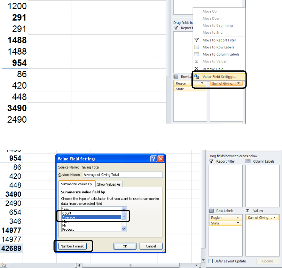
Changing Value Field Settings

If you would like the Pivot Table to show average donations instead of summing the donations,

you can click on “Sum of Giving Totals” under the “Value” area, then select” Value Field

Settings.”

You can then change the” Value” setting to “Average.”

Before clicking OK, you may wish to change the “Number Format” to “Currency” so that

numeric values will appear as dollar amounts.

After selecting “Number Format”, select “Currency” and make sure the “Decimal Places” are set

to 2. Click OK on both menus.

You will notice that donations are now displayed as averages and in currency format.

Pivot Tables - Slicers

Excel 2010 allows you to use the Slicer tool to filter your data. On the Pivot Table Tools

contextual ribbon, select “Insert Slicer.” In this example, we will check “Library” and click OK.

Holding the Ctrl button allows you to make multiple selections. In this case, the California

libraries have been selected in the Slicer tool. Notice that the Pivot Table now only shows

average donations to libraries in the Western region that are located in the state of California.

You can easily clear the filter by selecting the button in the upper right of the Slicer box.

Pivot Tables – Charts

Like other tables, Excel 2010 can easily convert a Pivot Table to a chart to display information in

a more visually interesting way. Simply click on the Insert ribbon, then select the kind of chart

you want.

Sparklines

Sparklines are a new feature in Excel 2010 that allow you to create a mini chart within a single

cell in order to show a visual representation of data trends.

Select the cell where you want your first Sparkline to appear, then select the Insert ribbon, then

“Line” under the “Sparklines” menu.

Then, highlight the data range, make sure the Sparkline location range is correct, then click OK.

A Sparkline chart appears showing a visual representation of that row’s data. You can then

AutoFill the rest of the rows.

You can easily change the look of your Sparklines or convert your line graphs to bar graphs

using the menu options on the Sparkline Tools Design contextual ribbon.

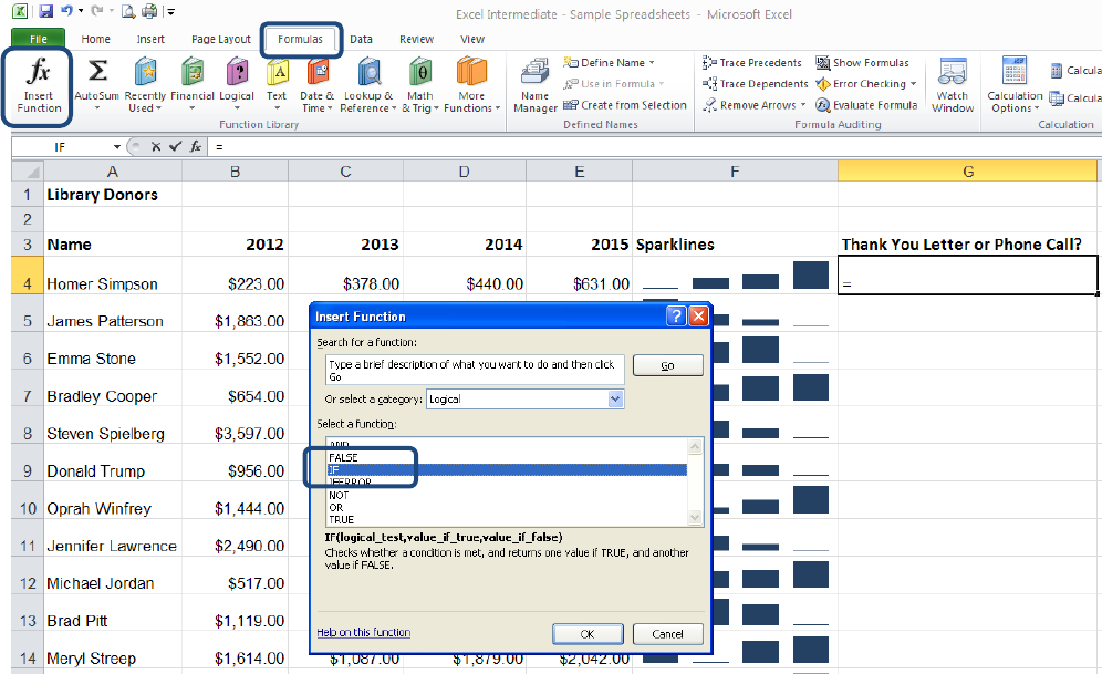
Logical Functions

Excel offers functions that compare data using logical operators such < (less than), > (greater

than), = (equal to), etc. In the example below, the logical function “IF” allows Excel to compare

donors’ 2014 donations amounts to their 2012 amounts and then indicate if that donor should

receive a thank you letter for increasing their donation or a phone call requesting additional

funding.

Select the Formulas ribbon, then “Insert Function.” Select the category “Logical” and then

select the “IF” function. Click OK.

In the “Logical_test” field, click on the cell with the 2014 donation amount, enter the > (greater

than) operator, click on the cell with the 2012 donation amount.

In the “Value_if_true” field, enter in quotations “Thank You Letter”.

In the “Value_if-false” field, enter in quotations “Phone Call”

Observe in the formula bar at the top how Excel constructs the function.

Click OK.

Excel then uses the logical function to determine that the first donor has given more in 2014

than in 2012 and indicates that this donor needs to receive a thank you letter.

Simply AutoFill the rest of the column and Excel applies the logical function to each donor.

Payment Function

Excel provides a simple way to calculate monthly loan payments using the Payment Function.

First, enter into a simple spreadsheet the price, interest rate, number of payments, and a blank

monthly payment line, like the example below.

Select the cell where you want the monthly payment calculation to go, select the Formulas

ribbon, and then the “Insert Function” option on the far left. An” Insert Function” dialog box

will appear. Search for the “Payment” function (abbreviated PMT) and click OK.

The “Function Argument”s box will appear. Click on the “Rate” field, then select the cell with

the interest rate amount.

In order to have Excel calculate the interest rate on a per-month basis, add a “/12” next to the

cell address.

For the “Nper” (number of payments) field, select the cell with the number of payments and for

the “Pv” (present value) field, select the cell with the item’s price. Lastly, click OK.

Excel will then display the monthly payment amount.

Once Excel completes the Payment Function, you can change the price, interest rate, and

number of payment values to see how it impacts the monthly payment amount.

VLOOKUP

The VLOOKUP function in Excel is a useful tool when you need to perform calculations that

reference a table with a range of values. This feature is frequently used when cross referencing

incomes with income tax ranges or, as in the example below, cross referencing sales revenues

with commission ranges.

Select the cell of the first commission rate, select the Formulas ribbon and then ”Insert

Function.” In the search field, type “VLOOKUP” and select it from the search results. Click OK.

In the ”Lookup_value” field, select the cell with revenue amount.

In the “Table_array” field, highlight the data in the revenue/commission table, excluding the

column headings.

Important: The “Table_array” range must then be converted to absolute values by entering a $

before each column letter and each row number.

In the” Col_index_num” field, enter the relative column number of the Commission data. This

table has three columns and the Commission data is in the third column, so enter 3.

Excel then cross references the salesperson’s revenue with the revenue/commission table and

determines the appropriate commission rate.

Use AutoFill to determine the commission rates of the other salespersons.

Calculating the commission paid to each sales person is a simple multiplication formula,

multiplying the Revenue cell with the Commission Rate cell.

AutoFill the remaining commissions.

External Cell Reference

It might be necessary to reference a cell from another worksheet within the workbook. An

example would be collecting quarterly totals into an annual report on a separate worksheet.

Say the quarterly budget totals are one worksheet and we want to add them together on a

separate worksheet.

Add the quarterly totals for all

four quarters (3

and 4th quarters

not shown) and display the results

in these cells

The formula looks like this:

Note that the source worksheet name has single quotes. This is because the worksheet name

contains a space.